Rate Equation
Objective
Define equation
Solve equation
Compute model and signal
Note
In this example, we only deal with gaussian irf
# import needed module
import numpy as np
import matplotlib.pyplot as plt
import TRXASprefitpack
from TRXASprefitpack import solve_model, solve_seq_model, solve_l_model, compute_model, rate_eq_conv
plt.rcParams["figure.figsize"] = (14,10)
Version information
print(TRXASprefitpack.__version__)
0.5.0
basic information of functions
help(solve_model)
Help on function solve_model in module TRXASprefitpack.mathfun.rate_eq:

solve_model(equation: numpy.ndarray, y0: numpy.ndarray) -> Tuple[numpy.ndarray, numpy.ndarray, numpy.ndarray]
    Solve system of first order rate equation

    Args:
      equation: matrix corresponding to model
      y0: initial condition

    Returns:
       1. eigenvalues of equation
       2. eigenvectors for equation
       3. coefficient where y0 = Vc
help(solve_l_model)
Help on function solve_l_model in module TRXASprefitpack.mathfun.rate_eq:

solve_l_model(equation: numpy.ndarray, y0: numpy.ndarray) -> Tuple[numpy.ndarray, numpy.ndarray, numpy.ndarray]
    Solve system of first order rate equation where the rate equation matrix is
    lower triangle

    Args:
      equation: matrix corresponding to model
      y0: initial condition

    Returns:
       1. eigenvalues of equation
       2. eigenvectors for equation
       3. coefficient where y0 = Vc
help(solve_seq_model)
Help on function solve_seq_model in module TRXASprefitpack.mathfun.rate_eq:

solve_seq_model(tau)
    Solve sequential decay model

    sequential decay model:
      0 -> 1 -> 2 -> 3 -> ... -> n
    initial condition:
     y0 = [1, 0, 0, ..., 0]

    Args:
      tau: liftime constants for each decay
      y0: initial condition

    Returns:
       1. eigenvalues of equation
       2. eigenvectors for equation
       3. coefficient to match initial condition
help(compute_model)
Help on function compute_model in module TRXASprefitpack.mathfun.rate_eq:

compute_model(t: numpy.ndarray, eigval: numpy.ndarray, V: numpy.ndarray, c: numpy.ndarray) -> numpy.ndarray
    Compute solution of the system of rate equations solved by solve_model
    Note: eigval, V, c should be obtained from solve_model

    Args:
     t: time
     eigval: eigenvalue for equation
     V: eigenvectors for equation
     c: coefficient

    Returns:
      solution of rate equation

    Note:
      eigval, V, c should be obtained from solve_model.
help(rate_eq_conv)
Help on function rate_eq_conv in module TRXASprefitpack.mathfun.exp_decay_fit:

rate_eq_conv(t: numpy.ndarray, fwhm: Union[float, numpy.ndarray], abs: numpy.ndarray, eigval: numpy.ndarray, V: numpy.ndarray, c: numpy.ndarray, irf: Union[str, NoneType] = 'g', eta: Union[float, NoneType] = None) -> numpy.ndarray
    Constructs signal model rate equation with
    instrumental response function
    Supported instrumental response function are

      * g: gaussian distribution
      * c: cauchy distribution
      * pv: pseudo voigt profile

    Args:
       t: time
       fwhm: full width at half maximum of instrumental response function
       abs: coefficient for each excited state
       eigval: eigenvalue of rate equation matrix
       V: eigenvector of rate equation matrix
       c: coefficient to match initial condition of rate equation
       irf: shape of instrumental
            response function [default: g]

              * 'g': normalized gaussian distribution,
              * 'c': normalized cauchy distribution,
              * 'pv': pseudo voigt profile :math:`(1-\eta)g + \eta c`
       eta: mixing parameter for pseudo voigt profile
            (only needed for pseudo voigt profile,
            default value is guessed according to
            Journal of Applied Crystallography. 33 (6): 1311–1316.)

    Returns:
      Convolution of the solution of the rate equation and instrumental
      response function.

    Note:
        *fwhm* For gaussian and cauchy distribution,
        only one value of fwhm is needed,
        so fwhm is assumed to be float
        However, for pseudo voigt profile,
        it needs two value of fwhm, one for gaussian part and
        the other for cauchy part.
        So, in this case,
        fwhm is assumed to be numpy.ndarray with size 2.
Define equation -sequential decay-
Note
In pump-probe time resolved spectroscopy, the concentration of ground state is not much important. Only, the concentration of excited species are matter.
Consider following sequential decay model
'''
    k1     k2
A  ---> B ---> GS
y1: A
y2: B
y3: GS
'''
with initial condition
Then what we need to solve is
with \(y(0)=y_0\).
Where \(A\) is
This type of 1st order rate equation can be solved via solve_seq_model
# set lifetime tau1 = 500 ps, tau2 = 10 ns
# set fwhm of IRF = 100 ps

tau_1 = 500
tau_2 = 10000
fwhm = 100

# initial condition
y0 = np.array([1, 0, 0])

# set time range (mixed step)
t_seq1 = np.arange(-2500, -500, 100)
t_seq2 = np.arange(-500, 1500, 50)
t_seq3 = np.arange(1500, 5000, 250)
t_seq4 = np.arange(5000, 50000, 2500)

t_seq = np.hstack((t_seq1, t_seq2, t_seq3, t_seq4))

eigval_seq, V_seq, c_seq = solve_seq_model(np.array([tau_1, tau_2]))
# Now compute model
y_seq = compute_model(t_seq, eigval_seq, V_seq, c_seq)


# since, y_1 + y_2 + y_3 = 1 for all t,
# y3 = 1 - (y_1+y_2)

y_seq[-1, :] = 1 - (y_seq[0, :] + y_seq[1, :])
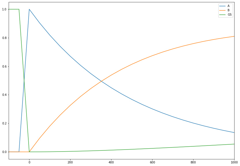
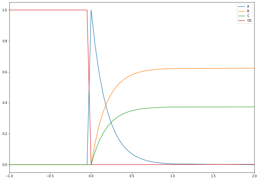
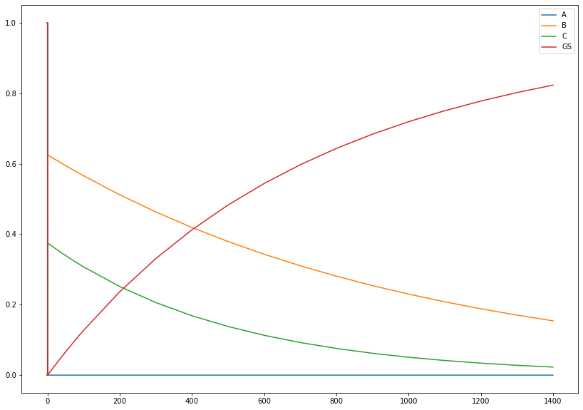
plot model (sequential decay model)
plt.plot(t_seq, y_seq[0, :], label='A')
plt.plot(t_seq, y_seq[1, :], label='B')
plt.plot(t_seq, y_seq[2, :], label='GS')
plt.xlim(-100, 1000)
plt.legend()
plt.show()
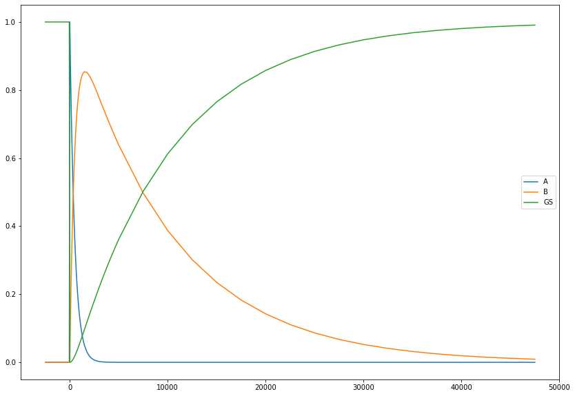
plt.plot(t_seq, y_seq[0, :], label='A')
plt.plot(t_seq, y_seq[1, :], label='B')
plt.plot(t_seq, y_seq[2, :], label='GS')
plt.legend()
plt.show()
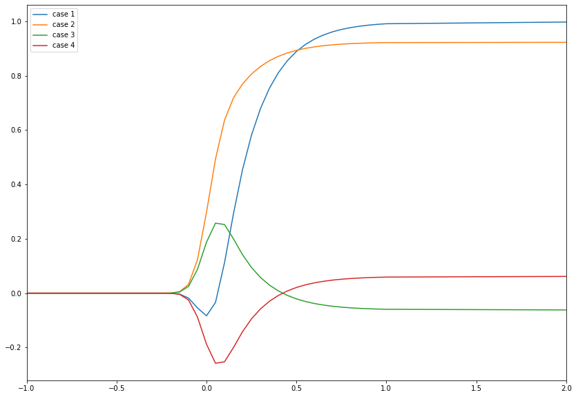
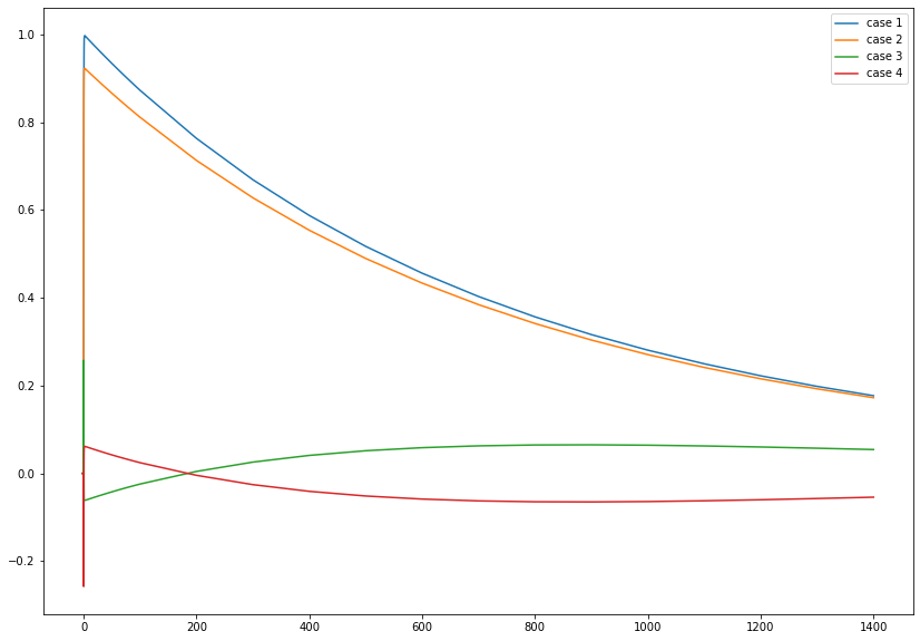
Compute Signal for sequential decay
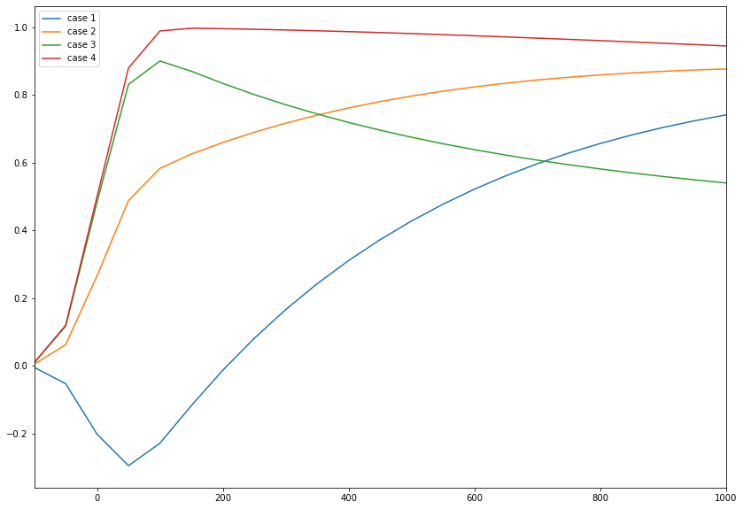
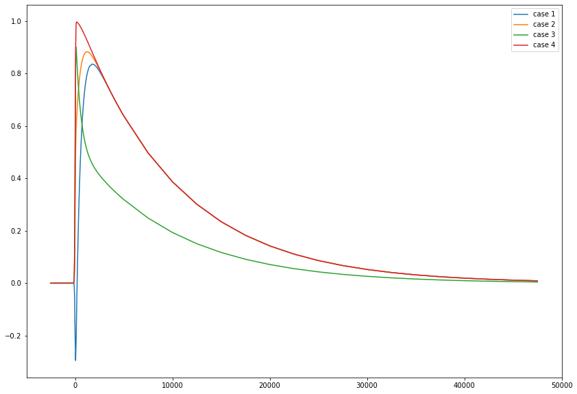
Difference absorption coefficient of ground state is 0
case 1. Differential absorption coefficient of A : -0.5 and B : 1
case 2. A: 0.5 B: 1
case 3. A: 1 B: 0.5
case 4. A: 1 B: 1
diff_abs_1 = [-0.5, # A state
            1, # B state
            0, # ground state
           ]
diff_abs_2 = [0.5, 1, 0]
diff_abs_3 = [1, 0.5, 0]
diff_abs_4 = [1, 1, 0]
y_seq_1 = rate_eq_conv(t_seq, fwhm, diff_abs_1, eigval_seq, V_seq, c_seq)
y_seq_2 = rate_eq_conv(t_seq, fwhm, diff_abs_2, eigval_seq, V_seq, c_seq)
y_seq_3 = rate_eq_conv(t_seq, fwhm, diff_abs_3, eigval_seq, V_seq, c_seq)
y_seq_4 = rate_eq_conv(t_seq, fwhm, diff_abs_4, eigval_seq, V_seq, c_seq)
Plot signal (sequential decay)
plt.plot(t_seq, y_seq_1, label='case 1')
plt.plot(t_seq, y_seq_2, label='case 2')
plt.plot(t_seq, y_seq_3, label='case 3')
plt.plot(t_seq, y_seq_4, label='case 4')
plt.xlim(-100, 1000)
plt.legend()
plt.show()
plt.plot(t_seq, y_seq_1, label='case 1')
plt.plot(t_seq, y_seq_2, label='case 2')
plt.plot(t_seq, y_seq_3, label='case 3')
plt.plot(t_seq, y_seq_4, label='case 4')
plt.legend()
plt.show()
Define equation -branched decay-
Note
In pump-probe time resolved spectroscopy, the concentration of ground state is not much important. Only, the concentration of excited species are matter.
Consider following branched decay model
'''
    k1     k3
A  ---> B ---> GS
 \
  \
k2 \
    \
     > C ---> GS
          k4
y1: A
y2: B
y3: C
y4: GS
'''
with initial condition
Then what we need to solve is
with \(y(0)=y_0\).
Where \(A\) is
As you can see the rate equation matrix A is lower triangle.
This lower triangle type 1st order rate equation can be solved via solve_l_model
# set lifetime tau1: 300 fs, tau2: 500 fs, tau3: 1 ns, tau 4: 500 ps
# set fwhm of IRF = 150 fs

tau_1 = 0.3
tau_2 = 0.5
tau_3 = 1000
tau_4 = 500
fwhm = 0.15

# initial condition
y0 = np.array([1, 0, 0, 0])

# rate equation matrix
A = np.array([[-(1/tau_1+1/tau_2), 0, 0, 0],
[1/tau_1, -1/tau_3, 0, 0],
[1/tau_2, 0, -1/tau_4, 0],
[0,1/tau_3, 1/tau_4, 0]
])


# set time range (mixed step)
t_1 = np.arange(-2, -1, 0.1)
t_2 = np.arange(-1, 1, 0.05)
t_3 = np.arange(1, 10, 1)
t_4 = np.arange(10, 100, 10)
t_5 = np.arange(100, 1500, 100)

t_branch = np.hstack((t_1, t_2, t_3, t_4, t_5))

eigval_branch, V_branch, c_branch = solve_l_model(A, y0)
# Now compute model
y_branch = compute_model(t_branch, eigval_branch, V_branch, c_branch)


# since, y_1 + y_2 + y_3 + y_4 = 1 for all t,
# y4 = 1 - (y_1+y_2+y_3)

y_branch[-1, :] = 1 - (y_branch[0, :] + y_branch[1, :] + y_branch[2, :])
plot model (branched decay model)
plt.plot(t_branch, y_branch[0, :], label='A')
plt.plot(t_branch, y_branch[1, :], label='B')
plt.plot(t_branch, y_branch[2, :], label='C')
plt.plot(t_branch, y_branch[3, :], label='GS')
plt.legend()
plt.xlim(-1, 2)
plt.show()
plt.plot(t_branch, y_branch[0, :], label='A')
plt.plot(t_branch, y_branch[1, :], label='B')
plt.plot(t_branch, y_branch[2, :], label='C')
plt.plot(t_branch, y_branch[3, :], label='GS')
plt.legend()
plt.show()
Compute Signal for branched decay
Difference absorption coefficient of ground state is 0
case 1. Differential absorption coefficient of A : -0.5 and B : 1 C: 1
case 2. A: 0.5 B: 1 C: 0.8
case 3. A: 0.5 B: 0.5 C: 1
case 4. A: -0.5 B: -0.5 C: 1
diff_abs_1 = [-0.5, # A state
            1, # B state
            1, # C
            0, # Ground State
           ]
diff_abs_2 = [0.5, 1, 0.8, 0]
diff_abs_3 = [0.5, 0.5, -1, 0]
diff_abs_4 = [-0.5, -0.5, 1, 0]
y_branch_1 = rate_eq_conv(t_branch, fwhm, diff_abs_1, eigval_branch, V_branch, c_branch)
y_branch_2 = rate_eq_conv(t_branch, fwhm, diff_abs_2, eigval_branch, V_branch, c_branch)
y_branch_3 = rate_eq_conv(t_branch, fwhm, diff_abs_3, eigval_branch, V_branch, c_branch)
y_branch_4 = rate_eq_conv(t_branch, fwhm, diff_abs_4, eigval_branch, V_branch, c_branch)
Plot Signal for branched decay
plt.plot(t_branch, y_branch_1, label='case 1')
plt.plot(t_branch, y_branch_2, label='case 2')
plt.plot(t_branch, y_branch_3, label='case 3')
plt.plot(t_branch, y_branch_4, label='case 4')
plt.legend()
plt.xlim(-1, 2)
plt.show()
plt.plot(t_branch, y_branch_1, label='case 1')
plt.plot(t_branch, y_branch_2, label='case 2')
plt.plot(t_branch, y_branch_3, label='case 3')
plt.plot(t_branch, y_branch_4, label='case 4')
plt.legend()
plt.show()
Conclusion
This example introduce solve_seq_model and solve_l_model to solve special kind of rate equation and demonstrates how signal changes when varying differential absolution coefficients of each excited state species.