Dampled Oscillation
Objective
Demonstrates dmp_osc_conv_gau, dmp_osc_conv_cauchy, dmp_osc_conv_pvoigt routine
dmp_osc_conv_gau: Computes the convolution of damped oscillation and gaussian function
dmp_osc_conv_cauchy: Computes the convolution of damped oscillation and cauchy function
dmp_osc_conv_pvoigt: Computes the convolution of damped oscillation and pseudo voigt function
Dampled oscillation is modeled to \(\exp(-kt)\cos(2\pi t/T+\phi)\)
import numpy as np
import matplotlib.pyplot as plt
from TRXASprefitpack import dmp_osc_conv_gau, dmp_osc_conv_cauchy, dmp_osc_conv_pvoigt
plt.rcParams["figure.figsize"] = (14,10)
Condition
fwhm: 0.15 pstau: 10 psperiod: 0.15 ps 0.3 ps 3 psphase: 0eta: 0.3
fwhm = 0.15
tau = 10
period = [0.15, 0.3, 3]
phase_factor = 0
eta = 0.3

# time range
t_0 = np.arange(-2, -1, 0.2)
t_1 = np.arange(-1, 1, 0.1)
t_2 = np.arange(1, 3, 0.2)
t_3 = np.arange(3, 10, 0.5)
t_4 = np.arange(10, 50, 4)
t_5 = np.arange(50, 100, 10)
t_6 = np.arange(100, 1100, 100)

t = np.hstack((t_0, t_1, t_2, t_3, t_4, t_5, t_6))
dmp_osc_conv_gau routine
help(dmp_osc_conv_gau)
Help on function dmp_osc_conv_gau in module TRXASprefitpack.mathfun.exp_conv_irf:

dmp_osc_conv_gau(t: Union[float, numpy.ndarray], fwhm: float, k: float, T: float, phase: float) -> Union[float, numpy.ndarray]
    Compute damped oscillation convolved with normalized gaussian
    distribution

    Args:
      t: time
      fwhm: full width at half maximum of gaussian distribution
      k: damping constant (inverse of life time)
      T: period of vibration
      phase: phase factor

    Returns:
     Convolution of normalized gaussian distribution and
     damped oscillation :math:`(\exp(-kt)cos(2\pi t/T+phase))`.
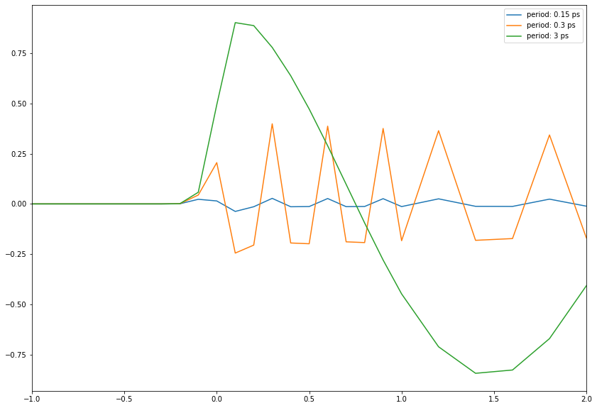
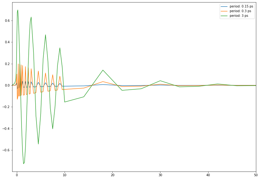
gau_osc_1 = dmp_osc_conv_gau(t, fwhm, 1/tau, period[0], phase_factor)
gau_osc_2 = dmp_osc_conv_gau(t, fwhm, 1/tau, period[1], phase_factor)
gau_osc_3 = dmp_osc_conv_gau(t, fwhm, 1/tau, period[2], phase_factor)
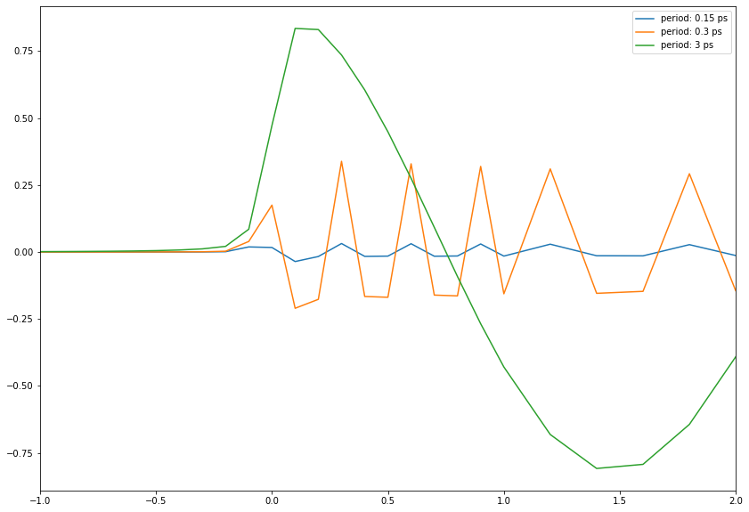
plt.plot(t, gau_osc_1, label=f'period: {period[0]} ps')
plt.plot(t, gau_osc_2, label=f'period: {period[1]} ps')
plt.plot(t, gau_osc_3, label=f'period: {period[2]} ps')
plt.legend()
plt.xlim(-1, 2)
plt.show()
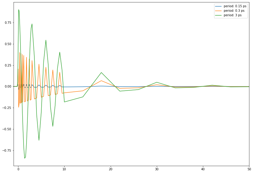
plt.plot(t, gau_osc_1, label=f'period: {period[0]} ps')
plt.plot(t, gau_osc_2, label=f'period: {period[1]} ps')
plt.plot(t, gau_osc_3, label=f'period: {period[2]} ps')
plt.legend()
plt.xlim(-1,50)
plt.show()
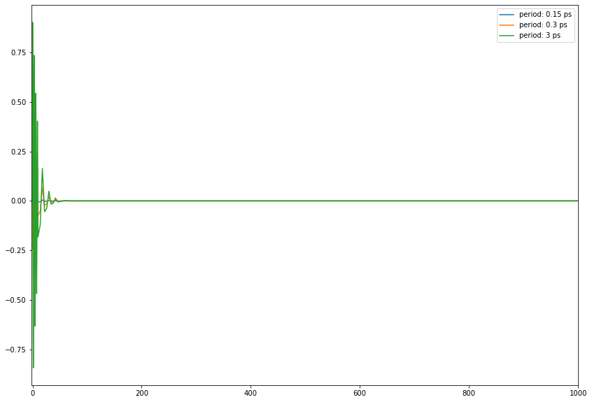
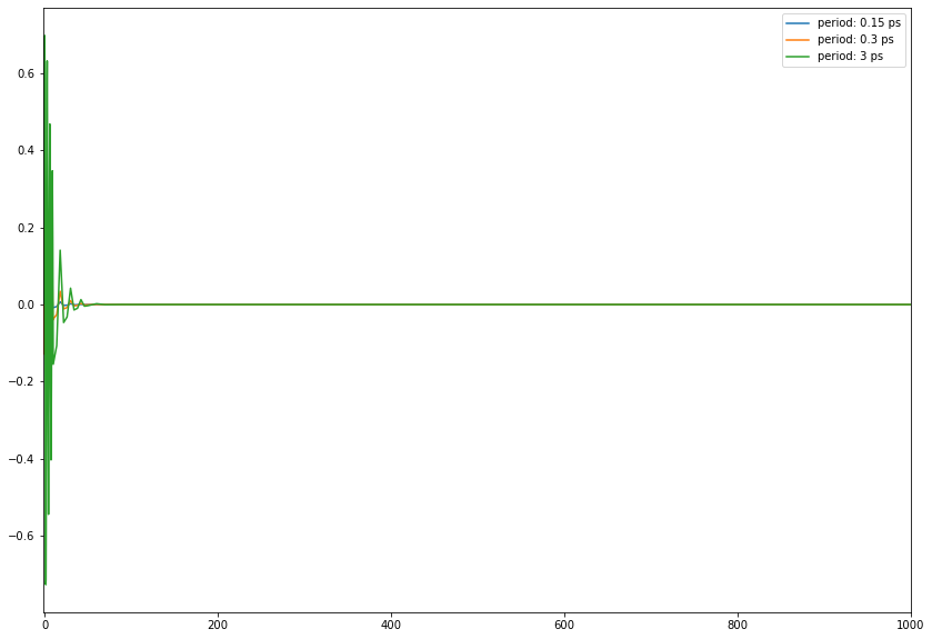
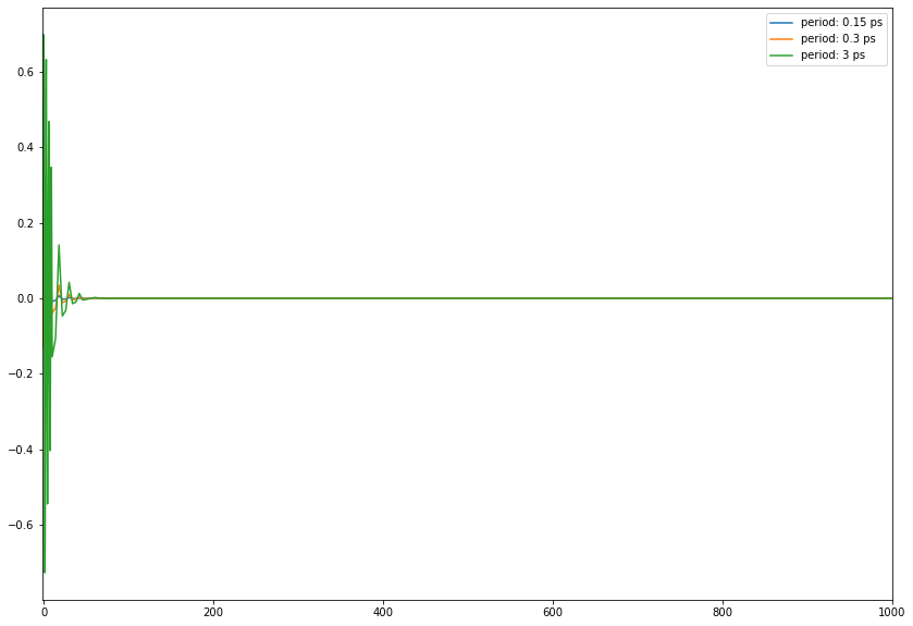
plt.plot(t, gau_osc_1, label=f'period: {period[0]} ps')
plt.plot(t, gau_osc_2, label=f'period: {period[1]} ps')
plt.plot(t, gau_osc_3, label=f'period: {period[2]} ps')
plt.legend()
plt.xlim(-2, 1000)
plt.show()
dmp_osc_conv_cauchy routine
help(dmp_osc_conv_cauchy)
Help on function dmp_osc_conv_cauchy in module TRXASprefitpack.mathfun.exp_conv_irf:

dmp_osc_conv_cauchy(t: Union[float, numpy.ndarray], fwhm: float, k: float, T: float, phase: float) -> Union[float, numpy.ndarray]
    Compute damped oscillation convolved with normalized cauchy
    distribution

    Args:
      t: time
      fwhm: full width at half maximum of cauchy distribution
      k: damping constant (inverse of life time)
      T: period of vibration
      phase: phase factor

    Returns:
     Convolution of normalized cauchy distribution and
     damped oscillation :math:`(\exp(-kt)cos(2\pi t/T+phase))`.
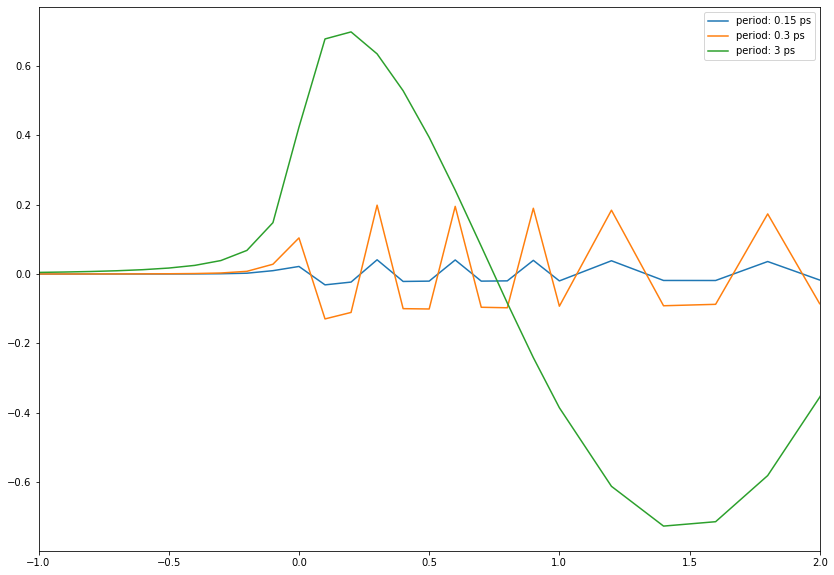
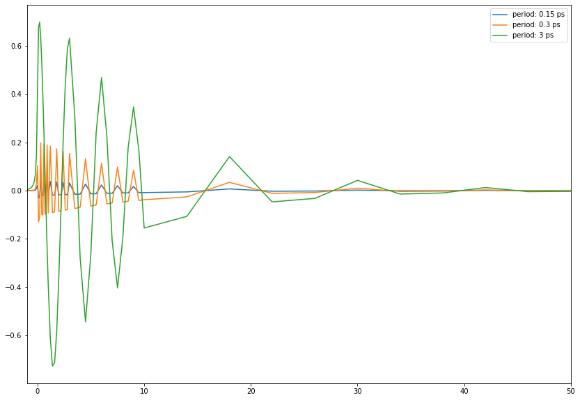
cauchy_osc_1 = dmp_osc_conv_cauchy(t, fwhm, 1/tau, period[0], phase_factor)
cauchy_osc_2 = dmp_osc_conv_cauchy(t, fwhm, 1/tau, period[1], phase_factor)
cauchy_osc_3 = dmp_osc_conv_cauchy(t, fwhm, 1/tau, period[2], phase_factor)
plt.plot(t, cauchy_osc_1, label=f'period: {period[0]} ps')
plt.plot(t, cauchy_osc_2, label=f'period: {period[1]} ps')
plt.plot(t, cauchy_osc_3, label=f'period: {period[2]} ps')
plt.legend()
plt.xlim(-1, 2)
plt.show()
plt.plot(t, cauchy_osc_1, label=f'period: {period[0]} ps')
plt.plot(t, cauchy_osc_2, label=f'period: {period[1]} ps')
plt.plot(t, cauchy_osc_3, label=f'period: {period[2]} ps')
plt.legend()
plt.xlim(-1, 50)
plt.show()
plt.plot(t, cauchy_osc_1, label=f'period: {period[0]} ps')
plt.plot(t, cauchy_osc_2, label=f'period: {period[1]} ps')
plt.plot(t, cauchy_osc_3, label=f'period: {period[2]} ps')
plt.legend()
plt.xlim(-2, 1000)
plt.show()
dmp_osc_conv_pvoigt
help(dmp_osc_conv_pvoigt)
Help on function dmp_osc_conv_pvoigt in module TRXASprefitpack.mathfun.exp_conv_irf:

dmp_osc_conv_pvoigt(t: Union[float, numpy.ndarray], fwhm_G: float, fwhm_L: float, eta: float, k: float, T: float, phase: float) -> Union[float, numpy.ndarray]
    Compute damped oscillation convolved with normalized pseudo
    voigt profile (i.e. linear combination of normalized gaussian and
    cauchy distribution)

    :math:`\eta C(\mathrm{fwhm}_L, t) + (1-\eta)G(\mathrm{fwhm}_G, t)`

    Args:
       t: time
       fwhm_G: full width at half maximum of gaussian part of
               pseudo voigt profile
       fwhm_L: full width at half maximum of cauchy part of
               pseudo voigt profile
       eta: mixing parameter
       k: damping constant (inverse of life time)
       T: period of vibration
       phase: phase factor

    Returns:
     Convolution of normalized pseudo voigt profile and
     damped oscillation :math:`(\exp(-kt)cos(2\pi t/T+phase))`.
pvoigt_osc_1 = dmp_osc_conv_pvoigt(t, fwhm, fwhm, eta, 1/tau, period[0], phase_factor)
pvoigt_osc_2 = dmp_osc_conv_pvoigt(t, fwhm, fwhm, eta, 1/tau, period[1], phase_factor)
pvoigt_osc_3 = dmp_osc_conv_pvoigt(t, fwhm, fwhm, eta, 1/tau, period[2], phase_factor)
plt.plot(t, pvoigt_osc_1, label=f'period: {period[0]} ps')
plt.plot(t, pvoigt_osc_2, label=f'period: {period[1]} ps')
plt.plot(t, pvoigt_osc_3, label=f'period: {period[2]} ps')
plt.legend()
plt.xlim(-1, 2)
plt.show()
plt.plot(t, cauchy_osc_1, label=f'period: {period[0]} ps')
plt.plot(t, cauchy_osc_2, label=f'period: {period[1]} ps')
plt.plot(t, cauchy_osc_3, label=f'period: {period[2]} ps')
plt.legend()
plt.xlim(-1, 50)
plt.show()
plt.plot(t, cauchy_osc_1, label=f'period: {period[0]} ps')
plt.plot(t, cauchy_osc_2, label=f'period: {period[1]} ps')
plt.plot(t, cauchy_osc_3, label=f'period: {period[2]} ps')
plt.legend()
plt.xlim(-2, 1000)
plt.show()
Conclusion
When the value of
periodof oscillation is similar to or less thanfwhmof gaussian probe pulse, It is hard to see oscillation feature.Shown as
IRFexample, the shape of the convolution of cauchy irf and damped oscilliation is much broader than that of gaussian irf one.Eventhough
phaseis 0, the oscillation peak near0is not the highest one when oscillation periodTis comparable tofwhm