Fitting with Static spectrum (Model: Voigt)
Objective
Fitting with sum of voigt profile model
Save and Load fitting result
Retrieve or interpolate experimental spectrum based on fitting result and calculates its derivative up to 2.
# import needed module
import numpy as np
import matplotlib.pyplot as plt
import TRXASprefitpack
from TRXASprefitpack import voigt, edge_gaussian
plt.rcParams["figure.figsize"] = (12,9)
Version information
print(TRXASprefitpack.__version__)
0.7.0
# Generates fake experiment data
# Model: sum of 3 voigt profile and one gaussian edge fature
e0_1 = 8987
e0_2 = 9000
e0_edge = 8992
fwhm_G_1 = 0.8
fwhm_G_2 = 0.9
fwhm_L_1 = 3
fwhm_L_2 = 9
fwhm_edge = 7
# set scan range
e = np.linspace(8960, 9020, 160)
# generate model spectrum
model_static = 0.1*voigt(e-e0_1, fwhm_G_1, fwhm_L_1) + \
0.7*voigt(e-e0_2, fwhm_G_2, fwhm_L_2) + \
0.2*edge_gaussian(e-e0_edge, fwhm_edge)
# set noise level
eps = 1/1000
# generate random noise
noise_static = np.random.normal(0, eps, model_static.size)
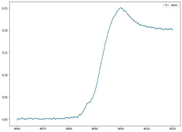
# generate measured static spectrum
obs_static = model_static + noise_static
eps_static = eps*np.ones_like(model_static)
# plot model experimental data

plt.errorbar(e, obs_static, eps_static, label='static')
plt.legend()
plt.show()
# import needed module for fitting
from TRXASprefitpack import fit_static_voigt

# set initial guess
e0_init = np.array([9000]) # initial peak position
fwhm_G_init = np.array([0]) # fwhm_G = 0 -> lorenzian
fwhm_L_init = np.array([8])

e0_edge = np.array([8995]) # initial edge position
fwhm_edge = np.array([15]) # initial edge width

fit_result_static = fit_static_voigt(e0_init, fwhm_G_init, fwhm_L_init,
 edge='g', edge_pos_init=e0_edge,
 edge_fwhm_init = fwhm_edge, method_glb='ampgo',
 e=e, intensity=obs_static, eps=eps_static)
# print fitting result
print(fit_result_static)
[Model information]
    model : voigt
    edge: g

[Optimization Method]
    global: ampgo
    leastsq: trf

[Optimization Status]
    nfev: 1232
    status: 0
    global_opt msg: Requested Number of global iteration is finished.
    leastsq_opt msg: `xtol` termination condition is satisfied.

[Optimization Results]
    Data points: 160
    Number of effective parameters: 6
    Degree of Freedom: 154
    Chi squared:  935.4703
    Reduced chi squared:  6.0745
    AIC (Akaike Information Criterion statistic):  294.5401
    BIC (Bayesian Information Criterion statistic):  312.9911

[Parameters]
    e0_1:  8998.89155596 +/-  0.15177781 ( 0.00%)
    fwhm_(G, 1):  0.00000000 +/-  0.00000000 ( 0.00%)
    fwhm_(L, 1):  11.11029381 +/-  0.35637699 ( 3.21%)
    E0_(g, 1):  8992.33183991 +/-  0.08150217 ( 0.00%)
    fwhm_(G, edge, 1):  8.74897986 +/-  0.14862299 ( 1.70%)

[Parameter Bound]
    e0_1:  8992 <=  8998.89155596 <=  9008
    fwhm_(G, 1):  0 <=  0.00000000 <=  0
    fwhm_(L, 1):  4 <=  11.11029381 <=  16
    E0_(g, 1):  8965 <=  8992.33183991 <=  9025
    fwhm_(G, edge, 1):  7.5 <=  8.74897986 <=  30

[Component Contribution]
    Static spectrum
     voigt 1:  83.32%
     g type edge 1:  16.68%

[Parameter Correlation]
    Parameter Correlations >  0.1 are reported.
    (fwhm_(L, 1), e0_1) = -0.21
    (E0_(g, 1), e0_1) = -0.838
    (E0_(g, 1), fwhm_(L, 1)) =  0.468
    (fwhm_(G, edge, 1), e0_1) = -0.53
    (fwhm_(G, edge, 1), fwhm_(L, 1)) = -0.314
    (fwhm_(G, edge, 1), E0_(g, 1)) =  0.428
Using static_spectrum function in TRXASprefitpack, you can directly evaluates fitted static spectrum from fitting result
# plot fitting result and experimental data
from TRXASprefitpack import static_spectrum

plt.errorbar(e, obs_static, eps_static, label=f'expt', color='black')
plt.errorbar(e, static_spectrum(e, fit_result_static), label=f'fit', color='red')

plt.legend()
plt.show()
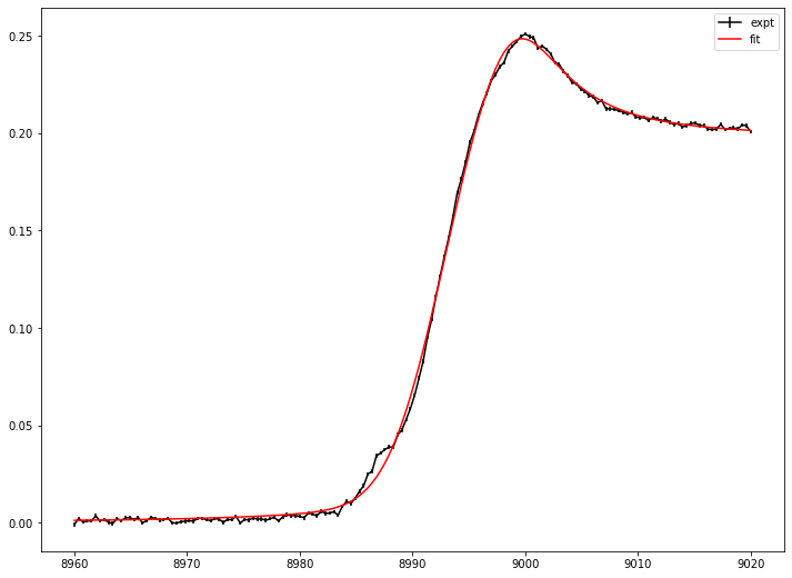
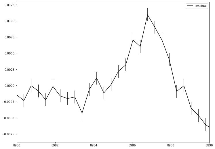
There exists one more peak near 8985 eV Region. To check this peak feature plot residual.
# plot residual

plt.errorbar(e, obs_static-static_spectrum(e, fit_result_static), eps_static, label=f'residual', color='black')

plt.legend()
plt.xlim(8980, 8990)
plt.show()
# try with two voigt feature
# set initial guess from previous fitting result and
# current observation

# set initial guess
e0_init = np.array([8987, 8999]) # initial peak position
fwhm_G_init = np.array([0, 0]) # fwhm_G = 0 -> lorenzian
fwhm_L_init = np.array([3, 11])

e0_edge = np.array([8992.3]) # initial edge position
fwhm_edge = np.array([9]) # initial edge width

fit_result_static_2 = fit_static_voigt(e0_init, fwhm_G_init, fwhm_L_init,
 edge='g', edge_pos_init=e0_edge,
 edge_fwhm_init = fwhm_edge, method_glb='ampgo',
 kwargs_lsq={'verbose' : 2},
 e=e, intensity=obs_static, eps=eps_static)
   Iteration     Total nfev        Cost      Cost reduction    Step norm     Optimality
       0              1         8.5728e+01                                    2.11e-03
       1              2         8.5728e+01      0.00e+00       0.00e+00       2.11e-03
`xtol` termination condition is satisfied.
Function evaluations 2, initial cost 8.5728e+01, final cost 8.5728e+01, first-order optimality 2.11e-03.
# print fitting result
print(fit_result_static_2)
[Model information]
    model : voigt
    edge: g

[Optimization Method]
    global: ampgo
    leastsq: trf

[Optimization Status]
    nfev: 2308
    status: 0
    global_opt msg: Requested Number of global iteration is finished.
    leastsq_opt msg: Both `ftol` and `xtol` termination conditions are satisfied.

[Optimization Results]
    Data points: 160
    Number of effective parameters: 9
    Degree of Freedom: 151
    Chi squared:  171.4556
    Reduced chi squared:  1.1355
    AIC (Akaike Information Criterion statistic):  29.0641
    BIC (Bayesian Information Criterion statistic):  56.7406

[Parameters]
    e0_1:  8987.11662114 +/-  0.05665087 ( 0.00%)
    e0_2:  9000.01345555 +/-  0.05284482 ( 0.00%)
    fwhm_(G, 1):  0.00000000 +/-  0.00000000 ( 0.00%)
    fwhm_(G, 2):  0.00000000 +/-  0.00000000 ( 0.00%)
    fwhm_(L, 1):  3.19604134 +/-  0.17792758 ( 5.57%)
    fwhm_(L, 2):  9.01582626 +/-  0.18757813 ( 2.08%)
    E0_(g, 1):  8992.02833484 +/-  0.01906209 ( 0.00%)
    fwhm_(G, edge, 1):  6.89941582 +/-  0.08112256 ( 1.18%)

[Parameter Bound]
    e0_1:  8984 <=  8987.11662114 <=  8990
    e0_2:  8988 <=  9000.01345555 <=  9010
    fwhm_(G, 1):  0 <=  0.00000000 <=  0
    fwhm_(G, 2):  0 <=  0.00000000 <=  0
    fwhm_(L, 1):  1.5 <=  3.19604134 <=  6
    fwhm_(L, 2):  5.5 <=  9.01582626 <=  22
    E0_(g, 1):  8974.3 <=  8992.02833484 <=  9010.3
    fwhm_(G, edge, 1):  4.5 <=  6.89941582 <=  18

[Component Contribution]
    Static spectrum
     voigt 1:  10.47%
     voigt 2:  69.73%
     g type edge 1:  19.80%

[Parameter Correlation]
    Parameter Correlations >  0.1 are reported.
    (e0_2, e0_1) =  0.274
    (fwhm_(L, 1), e0_1) =  0.401
    (fwhm_(L, 1), e0_2) =  0.374
    (fwhm_(L, 2), e0_1) = -0.182
    (fwhm_(L, 2), e0_2) = -0.511
    (fwhm_(L, 2), fwhm_(L, 1)) = -0.417
    (E0_(g, 1), e0_1) =  0.273
    (E0_(g, 1), e0_2) = -0.427
    (E0_(g, 1), fwhm_(L, 1)) =  0.18
    (E0_(g, 1), fwhm_(L, 2)) =  0.483
    (fwhm_(G, edge, 1), e0_1) = -0.522
    (fwhm_(G, edge, 1), e0_2) = -0.696
    (fwhm_(G, edge, 1), fwhm_(L, 1)) = -0.563
    (fwhm_(G, edge, 1), fwhm_(L, 2)) =  0.533
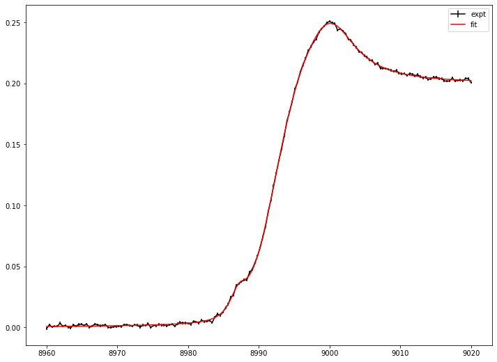
# plot fitting result and experimental data

plt.errorbar(e, obs_static, eps_static, label=f'expt', color='black')
plt.errorbar(e, static_spectrum(e, fit_result_static_2), label=f'fit', color='red')

plt.legend()
plt.show()
# save and load fitting result
from TRXASprefitpack import save_StaticResult, load_StaticResult

save_StaticResult(fit_result_static_2, 'static_example_voigt') # save fitting result to static_example_voigt.h5
loaded_result = load_StaticResult('static_example_voigt') # load fitting result from static_example_voigt.h5
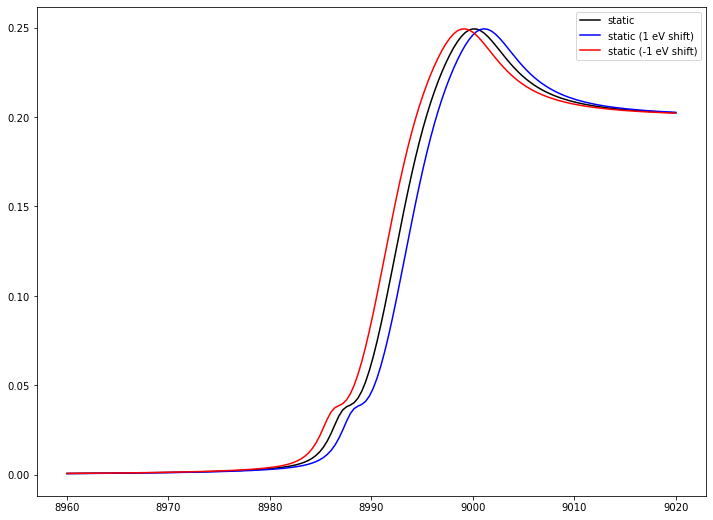
# plot static spectrum
plt.plot(e, static_spectrum(e, loaded_result), label='static', color='black')
plt.plot(e, static_spectrum(e-1, loaded_result), label='static (1 eV shift)', color='blue')
plt.plot(e, static_spectrum(e+1, loaded_result), label='static (-1 eV shift)', color='red')
plt.legend()
plt.show()
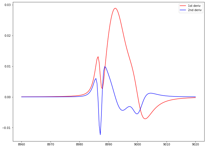
# plot its derivative up to second
plt.plot(e, static_spectrum(e, loaded_result, deriv_order=1), label='1st deriv', color='red')
plt.plot(e, static_spectrum(e, loaded_result, deriv_order=2), label='2nd deriv', color='blue')
plt.legend()
plt.show()
Optionally, you can calculated F-test based confidence interval
from TRXASprefitpack import confidence_interval

ci_result = confidence_interval(loaded_result, 0.05) # set significant level: 0.05 -> 95% confidence level
print(ci_result) # report confidence interval
[Report for Confidence Interval]
    Method: f
    Significance level:  5.000000e-02

[Confidence interval]
    8987.11662114 -  0.11434804 <= e0_1 <=  8987.11662114 +  0.11972999
    9000.01345555 -  0.10823585 <= e0_2 <=  9000.01345555 +  0.10126723
    3.19604134 -  0.34092248 <= fwhm_(L, 1) <=  3.19604134 +  0.36111441
    9.01582626 -  0.36170925 <= fwhm_(L, 2) <=  9.01582626 +  0.37766414
    8992.02833484 -  0.03728687 <= E0_(g, 1) <=  8992.02833484 +  0.03836275
    6.89941582 -  0.15987653 <= fwhm_(G, edge, 1) <=  6.89941582 +  0.16475738
# compare with ase
from scipy.stats import norm

factor = norm.ppf(1-0.05/2)

print('[Confidence interval (from ASE)]')
for i in range(loaded_result['param_name'].size):
    print(f"{loaded_result['x'][i] :.8f} - {factor*loaded_result['x_eps'][i] :.8f}",
          f"<= {loaded_result['param_name'][i]} <=", f"{loaded_result['x'][i] :.8f} + {factor*loaded_result['x_eps'][i] :.8f}")
[Confidence interval (from ASE)]
8987.11662114 - 0.11103366 <= e0_1 <= 8987.11662114 + 0.11103366
9000.01345555 - 0.10357394 <= e0_2 <= 9000.01345555 + 0.10357394
0.00000000 - 0.00000000 <= fwhm_(G, 1) <= 0.00000000 + 0.00000000
0.00000000 - 0.00000000 <= fwhm_(G, 2) <= 0.00000000 + 0.00000000
3.19604134 - 0.34873165 <= fwhm_(L, 1) <= 3.19604134 + 0.34873165
9.01582626 - 0.36764638 <= fwhm_(L, 2) <= 9.01582626 + 0.36764638
8992.02833484 - 0.03736102 <= E0_(g, 1) <= 8992.02833484 + 0.03736102
6.89941582 - 0.15899730 <= fwhm_(G, edge, 1) <= 6.89941582 + 0.15899730
In many case, ASE does not much different from more sophisticated f-test based error estimation.