Fitting with Static spectrum (Model: theoretical spectrum)
Objective
Fitting with voigt broadened theoretical spectrum
Save and Load fitting result
Retrieve or interpolate experimental spectrum based on fitting result and calculates its derivative up to 2.
# import needed module
import numpy as np
import matplotlib.pyplot as plt
import TRXASprefitpack
from TRXASprefitpack import voigt_thy, edge_gaussian
plt.rcParams["figure.figsize"] = (12,9)
Version information
print(TRXASprefitpack.__version__)
0.7.0
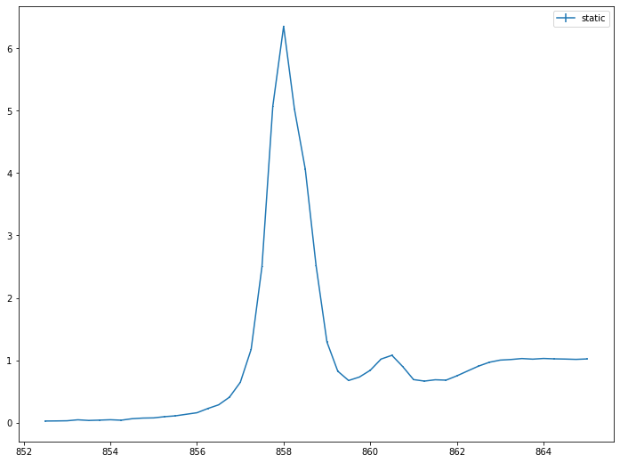
# Generates fake experiment data
# Model: sum of 2 normalized theoretical spectrum

edge_type = 'g'
e0_edge = np.array([860.5, 862])
fwhm_edge = np.array([1, 1.5])
peak_shift = np.array([862.5, 863])
mixing = np.array([0.3, 0.7])
mixing_edge = np.array([0.3, 0.7])
fwhm_G_thy = 0.3
fwhm_L_thy = 0.5

thy_peak = np.empty(2, dtype=object)
thy_peak[0] = np.genfromtxt('Ni_example_1.stk')
thy_peak[1] = np.genfromtxt('Ni_example_2.stk')

# set scan range
e = np.linspace(852.5, 865, 51)

# generate model spectrum
model_static = mixing[0]*voigt_thy(e, thy_peak[0], fwhm_G_thy, fwhm_L_thy,
peak_shift[0], policy='shift')+\
    mixing[1]*voigt_thy(e, thy_peak[1], fwhm_G_thy, fwhm_L_thy,
    peak_shift[1], policy='shift')+\
        mixing_edge[0]*edge_gaussian(e-e0_edge[0], fwhm_edge[0])+\
            mixing_edge[1]*edge_gaussian(e-e0_edge[1], fwhm_edge[1])

# set noise level
eps = 1/100
# generate random noise
noise_static = np.random.normal(0, eps, model_static.size)

# generate measured static spectrum
obs_static = model_static + noise_static
eps_static = eps*np.ones_like(model_static)
# plot model experimental data

plt.errorbar(e, obs_static, eps_static, label='static')
plt.legend()
plt.show()
Before fitting, we need to guess about initial peak shift paramter for theoretical spectrum
# Guess initial peak_shift
# check with arbitary fwhm paramter and peak_shift paramter
e_tst = np.linspace(-10, 20, 120)
comp_1 = voigt_thy(e_tst, thy_peak[0], 0.5, 1, 0, policy='shift')
comp_2 = voigt_thy(e_tst, thy_peak[1], 0.5, 1, 0, policy='shift')

plt.plot(e_tst, comp_1, label='comp_1')
plt.plot(e_tst, comp_2, label='comp_2')
plt.legend()
plt.show()
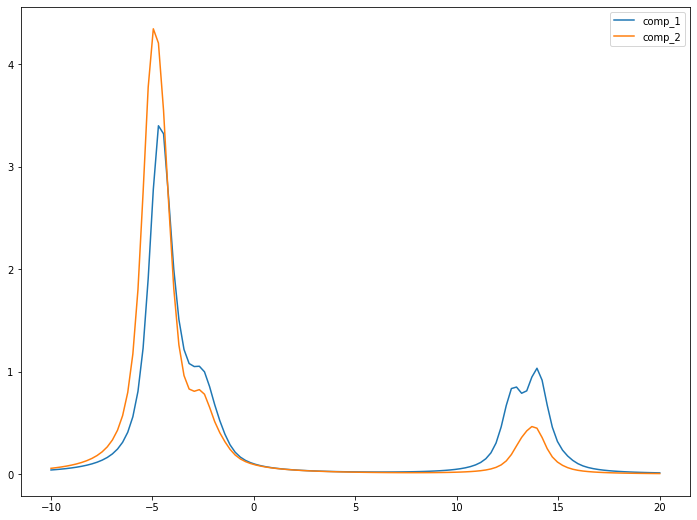
Compare first peak position, we can set initial peak shift paramter for both component as \(863\), \(863\). First try with only one component
from TRXASprefitpack import fit_static_thy
# initial guess
policy = 'shift'
peak_shift_init = np.array([863])
fwhm_G_thy_init = 0.5
fwhm_L_thy_init = 0.5

result_1 = fit_static_thy(thy_peak[:1], fwhm_G_thy_init, fwhm_L_thy_init,
policy, peak_shift_init, method_glb='ampgo',
e=e, intensity=obs_static, eps=eps_static)
/home/lis1331/anaconda3/lib/python3.8/site-packages/TRXASprefitpack/driver/_ampgo.py:372: RuntimeWarning: invalid value encountered in true_divide
  diff/dist
/home/lis1331/anaconda3/lib/python3.8/site-packages/TRXASprefitpack/driver/_ampgo.py:374: RuntimeWarning: divide by zero encountered in double_scalars
  y_ttf = numerator/denominator
/home/lis1331/anaconda3/lib/python3.8/site-packages/TRXASprefitpack/driver/_ampgo.py:375: RuntimeWarning: divide by zero encountered in true_divide
  deriv_y_ttf = 2*(grad_numerator/denominator +
print(result_1)
[Model information]
    model : thy
    policy: shift

[Optimization Method]
    global: ampgo
    leastsq: trf

[Optimization Status]
    nfev: 592
    status: 0
    global_opt msg: Requested Number of global iteration is finished.
    leastsq_opt msg: Both `ftol` and `xtol` termination conditions are satisfied.

[Optimization Results]
    Data points: 51
    Number of effective parameters: 4
    Degree of Freedom: 47
    Chi squared:  136411.8463
    Reduced chi squared:  2902.3797
    AIC (Akaike Information Criterion statistic):  410.472
    BIC (Bayesian Information Criterion statistic):  418.1993

[Parameters]
    fwhm_G:  0.52095336 +/-  0.31179381 ( 59.85%)
    fwhm_L:  0.53741688 +/-  0.23583688 ( 43.88%)
    peak_shift 1:  862.66584191 +/-  0.03366347 ( 0.00%)

[Parameter Bound]
    fwhm_G:  0.25 <=  0.52095336 <=  1
    fwhm_L:  0.25 <=  0.53741688 <=  1
    peak_shift 1:  862.18120204 <=  862.66584191 <=  863.81879796

[Component Contribution]
    Static spectrum
     thy 1:  100.00%

[Parameter Correlation]
    Parameter Correlations >  0.1 are reported.
    (fwhm_L, fwhm_G) = -0.919
Using static_spectrum function in TRXASprefitpack, you can directly evaluates fitted static spectrum from fitting result
# plot fitting result and experimental data
from TRXASprefitpack import static_spectrum

plt.errorbar(e, obs_static, eps_static, label=f'expt', color='black')
plt.errorbar(e, static_spectrum(e, result_1), label=f'fit', color='red')

plt.legend()
plt.show()
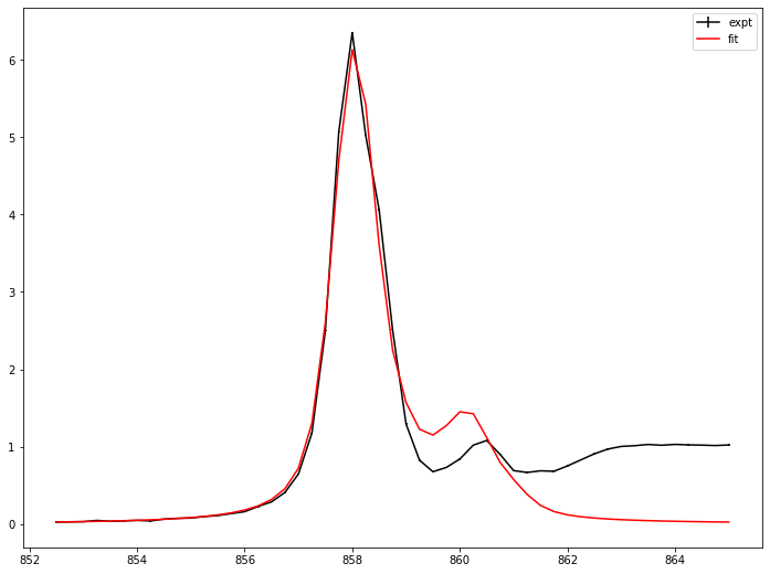
The fit looks not good, there may exists one more component.
# initial guess
# add one more thoeretical spectrum
policy = 'shift'
peak_shift_init = np.array([863, 863])
# Note that each thoeretical spectrum shares full width at half maximum paramter
fwhm_G_thy_init = 0.5
fwhm_L_thy_init = 0.5

result_2 = fit_static_thy(thy_peak, fwhm_G_thy_init, fwhm_L_thy_init,
policy, peak_shift_init, method_glb='ampgo',
e=e, intensity=obs_static, eps=eps_static)
/home/lis1331/anaconda3/lib/python3.8/site-packages/TRXASprefitpack/driver/_ampgo.py:372: RuntimeWarning: invalid value encountered in true_divide
  diff/dist
/home/lis1331/anaconda3/lib/python3.8/site-packages/TRXASprefitpack/driver/_ampgo.py:374: RuntimeWarning: divide by zero encountered in double_scalars
  y_ttf = numerator/denominator
/home/lis1331/anaconda3/lib/python3.8/site-packages/TRXASprefitpack/driver/_ampgo.py:375: RuntimeWarning: divide by zero encountered in true_divide
  deriv_y_ttf = 2*(grad_numerator/denominator +
print(result_2)
[Model information]
    model : thy
    policy: shift

[Optimization Method]
    global: ampgo
    leastsq: trf

[Optimization Status]
    nfev: 1392
    status: 0
    global_opt msg: Requested Number of global iteration is finished.
    leastsq_opt msg: Both `ftol` and `xtol` termination conditions are satisfied.

[Optimization Results]
    Data points: 51
    Number of effective parameters: 6
    Degree of Freedom: 45
    Chi squared:  119084.5932
    Reduced chi squared:  2646.3243
    AIC (Akaike Information Criterion statistic):  407.544
    BIC (Bayesian Information Criterion statistic):  419.1349

[Parameters]
    fwhm_G:  0.25000000 +/-  0.43872563 ( 175.49%)
    fwhm_L:  0.59975490 +/-  0.20534932 ( 34.24%)
    peak_shift 1:  862.59164170 +/-  0.23524873 ( 0.03%)
    peak_shift 2:  862.98150687 +/-  0.11346975 ( 0.01%)

[Parameter Bound]
    fwhm_G:  0.25 <=  0.25000000 <=  1
    fwhm_L:  0.25 <=  0.59975490 <=  1
    peak_shift 1:  862.18120204 <=  862.59164170 <=  863.81879796
    peak_shift 2:  862.18120204 <=  862.98150687 <=  863.81879796

[Component Contribution]
    Static spectrum
     thy 1:  33.40%
     thy 2:  66.60%

[Parameter Correlation]
    Parameter Correlations >  0.1 are reported.
    (fwhm_L, fwhm_G) = -0.885
    (peak_shift 1, fwhm_G) = -0.355
    (peak_shift 1, fwhm_L) =  0.491
    (peak_shift 2, fwhm_G) =  0.439
    (peak_shift 2, fwhm_L) = -0.542
    (peak_shift 2, peak_shift 1) = -0.855
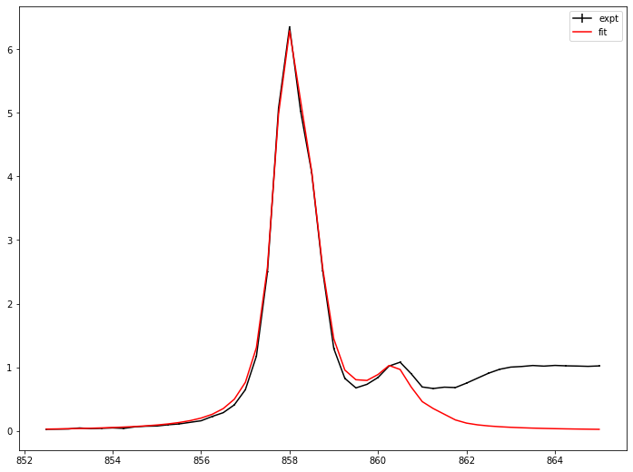
plt.errorbar(e, obs_static, eps_static, label=f'expt', color='black')
plt.errorbar(e, static_spectrum(e, result_2), label=f'fit', color='red')

plt.legend()
plt.show()
# plot residual
plt.errorbar(e, obs_static-static_spectrum(e, result_2), eps_static, label=f'res', color='red')

plt.legend()
plt.show()
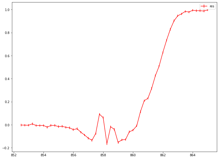
Residual suggests that there exists gaussian edge feature near 862 with fwhm 2
# try with two theoretical component and edge

# refine initial guess
policy = 'shift'
peak_shift_init = np.array([862.6, 863])
# Note that each thoeretical spectrum shares full width at half maximum paramter
fwhm_G_thy_init = 0.25
fwhm_L_thy_init = 0.5
# add one edge feature
e0_edge_init = np.array([862])
fwhm_edge_init = np.array([2])

result_2_edge = fit_static_thy(thy_peak, fwhm_G_thy_init, fwhm_L_thy_init,
policy, peak_shift_init,
edge='g', edge_pos_init=e0_edge_init,
edge_fwhm_init=fwhm_edge_init, method_glb='ampgo',
e=e, intensity=obs_static, eps=eps_static)
# print fitting result
print(result_2_edge)
[Model information]
    model : thy
    policy: shift
    edge: g

[Optimization Method]
    global: ampgo
    leastsq: trf

[Optimization Status]
    nfev: 3270
    status: 0
    global_opt msg: Requested Number of global iteration is finished.
    leastsq_opt msg: `xtol` termination condition is satisfied.

[Optimization Results]
    Data points: 51
    Number of effective parameters: 9
    Degree of Freedom: 42
    Chi squared:  89.9027
    Reduced chi squared:  2.1405
    AIC (Akaike Information Criterion statistic):  46.912
    BIC (Bayesian Information Criterion statistic):  64.2984

[Parameters]
    fwhm_G:  0.29976122 +/-  0.00865084 ( 2.89%)
    fwhm_L:  0.49960394 +/-  0.00633794 ( 1.27%)
    peak_shift 1:  862.50843083 +/-  0.00706934 ( 0.00%)
    peak_shift 2:  862.99673086 +/-  0.00299232 ( 0.00%)
    E0_g 1:  861.58687917 +/-  0.01733635 ( 0.00%)
    fwhm_(g, edge 1):  2.31987033 +/-  0.05701494 ( 2.46%)

[Parameter Bound]
    fwhm_G:  0.125 <=  0.29976122 <=  0.5
    fwhm_L:  0.25 <=  0.49960394 <=  1
    peak_shift 1:  861.99115937 <=  862.50843083 <=  863.20884063
    peak_shift 2:  862.39115937 <=  862.99673086 <=  863.60884063
    E0_g 1:  858 <=  861.58687917 <=  866
    fwhm_(g, edge 1):  1 <=  2.31987033 <=  4

[Component Contribution]
    Static spectrum
     thy 1:  14.27%
     thy 2:  35.38%
     g type edge 1:  50.35%

[Parameter Correlation]
    Parameter Correlations >  0.1 are reported.
    (fwhm_L, fwhm_G) = -0.848
    (peak_shift 1, fwhm_G) = -0.309
    (peak_shift 1, fwhm_L) =  0.599
    (peak_shift 2, fwhm_G) =  0.382
    (peak_shift 2, fwhm_L) = -0.599
    (peak_shift 2, peak_shift 1) = -0.682
    (E0_g 1, fwhm_G) = -0.144
    (E0_g 1, fwhm_L) =  0.191
    (E0_g 1, peak_shift 1) =  0.135
    (fwhm_(g, edge 1), fwhm_G) =  0.113
    (fwhm_(g, edge 1), fwhm_L) = -0.177
    (fwhm_(g, edge 1), peak_shift 1) = -0.18
    (fwhm_(g, edge 1), E0_g 1) =  0.211
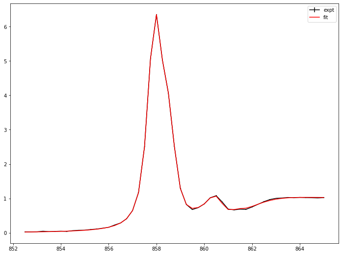
# plot fitting result and experimental data

plt.errorbar(e, obs_static, eps_static, label=f'expt', color='black')
plt.errorbar(e, static_spectrum(e, result_2_edge), label=f'fit', color='red')

plt.legend()
plt.show()
# plot residual
plt.errorbar(e, obs_static-static_spectrum(e, result_2_edge), eps_static, label=f'fit', color='red')

plt.legend()
plt.show()
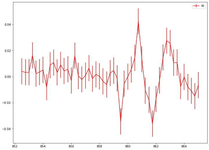
fit_static_thy supports adding multiple edge feature, to demenstrate this I add one more edge feature in the fitting model.
# add one more edge

# refine initial guess
policy = 'shift'
peak_shift_init = np.array([862.6, 863])
# Note that each thoeretical spectrum shares full width at half maximum paramter
fwhm_G_thy_init = 0.25
fwhm_L_thy_init = 0.5
# add one edge feature
e0_edge_init = np.array([860.5, 862])
fwhm_edge_init = np.array([0.8, 1.5])

result_2_edge_2 = fit_static_thy(thy_peak, fwhm_G_thy_init, fwhm_L_thy_init,
policy, peak_shift_init,
edge='g', edge_pos_init=e0_edge_init,
edge_fwhm_init=fwhm_edge_init, method_glb='ampgo',
e=e, intensity=obs_static, eps=eps_static)
print(result_2_edge_2)
[Model information]
    model : thy
    policy: shift
    edge: g

[Optimization Method]
    global: ampgo
    leastsq: trf

[Optimization Status]
    nfev: 6389
    status: 0
    global_opt msg: Requested Number of global iteration is finished.
    leastsq_opt msg: `xtol` termination condition is satisfied.

[Optimization Results]
    Data points: 51
    Number of effective parameters: 12
    Degree of Freedom: 39
    Chi squared:  23.0179
    Reduced chi squared:  0.5902
    AIC (Akaike Information Criterion statistic): -16.5732
    BIC (Bayesian Information Criterion statistic):  6.6087

[Parameters]
    fwhm_G:  0.29766541 +/-  0.00461112 ( 1.55%)
    fwhm_L:  0.50165657 +/-  0.00341226 ( 0.68%)
    peak_shift 1:  862.50861290 +/-  0.00383589 ( 0.00%)
    peak_shift 2:  862.99782704 +/-  0.00158692 ( 0.00%)
    E0_g 1:  861.96628745 +/-  0.04679976 ( 0.01%)
    E0_g 2:  860.44150114 +/-  0.06574437 ( 0.01%)
    fwhm_(g, edge 1):  1.54444699 +/-  0.08594562 ( 5.56%)
    fwhm_(g, edge 2):  1.01241472 +/-  0.13437182 ( 13.27%)

[Parameter Bound]
    fwhm_G:  0.125 <=  0.29766541 <=  0.5
    fwhm_L:  0.25 <=  0.50165657 <=  1
    peak_shift 1:  861.99115937 <=  862.50861290 <=  863.20884063
    peak_shift 2:  862.39115937 <=  862.99782704 <=  863.60884063
    E0_g 1:  858.9 <=  861.96628745 <=  862.1
    E0_g 2:  859 <=  860.44150114 <=  865
    fwhm_(g, edge 1):  0.4 <=  1.54444699 <=  1.6
    fwhm_(g, edge 2):  0.75 <=  1.01241472 <=  3

[Component Contribution]
    Static spectrum
     thy 1:  14.63%
     thy 2:  35.37%
     g type edge 1:  36.43%
     g type edge 2:  13.56%

[Parameter Correlation]
    Parameter Correlations >  0.1 are reported.
    (fwhm_L, fwhm_G) = -0.849
    (peak_shift 1, fwhm_G) = -0.334
    (peak_shift 1, fwhm_L) =  0.626
    (peak_shift 2, fwhm_G) =  0.373
    (peak_shift 2, fwhm_L) = -0.579
    (peak_shift 2, peak_shift 1) = -0.641
    (E0_g 1, fwhm_L) = -0.103
    (E0_g 1, peak_shift 1) = -0.104
    (E0_g 2, E0_g 1) =  0.924
    (fwhm_(g, edge 1), E0_g 1) = -0.891
    (fwhm_(g, edge 1), E0_g 2) = -0.827
    (fwhm_(g, edge 2), fwhm_G) =  0.137
    (fwhm_(g, edge 2), fwhm_L) = -0.218
    (fwhm_(g, edge 2), peak_shift 1) = -0.234
    (fwhm_(g, edge 2), E0_g 1) =  0.792
    (fwhm_(g, edge 2), E0_g 2) =  0.787
    (fwhm_(g, edge 2), fwhm_(g, edge 1)) = -0.664
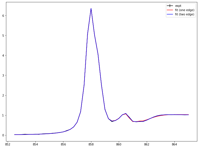
plt.errorbar(e, obs_static, eps_static, label=f'expt', color='black')
plt.errorbar(e, static_spectrum(e, result_2_edge), label=f'fit (one edge)', color='red')
plt.errorbar(e, static_spectrum(e, result_2_edge_2), label=f'fit (two edge)', color='blue')

plt.legend()
plt.show()
# save and load fitting result
from TRXASprefitpack import save_StaticResult, load_StaticResult

save_StaticResult(result_2_edge_2, 'static_example_thy') # save fitting result to static_example_thy.h5
loaded_result = load_StaticResult('static_example_thy') # load fitting result from static_example_thy.h5
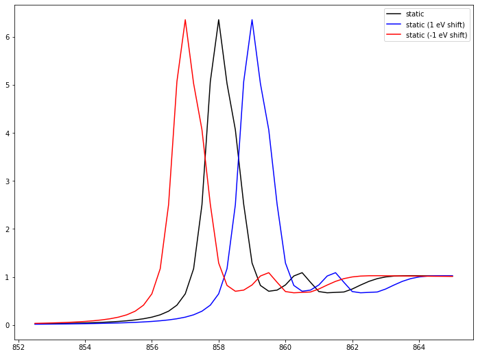
# plot static spectrum
plt.plot(e, static_spectrum(e, loaded_result), label='static', color='black')
plt.plot(e, static_spectrum(e-1, loaded_result), label='static (1 eV shift)', color='blue')
plt.plot(e, static_spectrum(e+1, loaded_result), label='static (-1 eV shift)', color='red')
plt.legend()
plt.show()
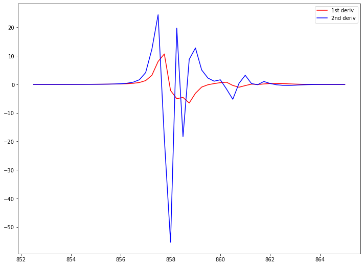
# plot its derivative up to second
plt.plot(e, static_spectrum(e, loaded_result, deriv_order=1), label='1st deriv', color='red')
plt.plot(e, static_spectrum(e, loaded_result, deriv_order=2), label='2nd deriv', color='blue')
plt.legend()
plt.show()
Optionally, you can calculated F-test based confidence interval
from TRXASprefitpack import confidence_interval

ci_result = confidence_interval(loaded_result, 0.05) # set significant level: 0.05 -> 95% confidence level
print(ci_result) # report confidence interval
[Report for Confidence Interval]
    Method: f
    Significance level:  5.000000e-02

[Confidence interval]
    0.29766541 -  0.00938656 <= fwhm_G <=  0.29766541 +  0.00919695
    0.50165657 -  0.0068657 <= fwhm_L <=  0.50165657 +  0.00680902
    862.5086129 -  0.00760942 <= peak_shift 1 <=  862.5086129 +  0.00763833
    862.99782704 -  0.00318677 <= peak_shift 2 <=  862.99782704 +  0.00321782
    861.96628745 -  0.06236662 <= E0_g 1 <=  861.96628745 +  0.11029989
    860.44150114 -  0.09856797 <= E0_g 2 <=  860.44150114 +  0.16654756
    1.54444699 -  0.182611 <= fwhm_(g, edge 1) <=  1.54444699 +  0.16610969
    1.01241472 -  0.21350814 <= fwhm_(g, edge 2) <=  1.01241472 +  0.29339317
# compare with ase
from scipy.stats import norm

factor = norm.ppf(1-0.05/2)

print('[Confidence interval (from ASE)]')
for i in range(loaded_result['param_name'].size):
    print(f"{loaded_result['x'][i] :.8f} - {factor*loaded_result['x_eps'][i] :.8f}",
          f"<= {loaded_result['param_name'][i]} <=", f"{loaded_result['x'][i] :.8f} + {factor*loaded_result['x_eps'][i] :.8f}")
[Confidence interval (from ASE)]
0.29766541 - 0.00903763 <= fwhm_G <= 0.29766541 + 0.00903763
0.50165657 - 0.00668791 <= fwhm_L <= 0.50165657 + 0.00668791
862.50861290 - 0.00751821 <= peak_shift 1 <= 862.50861290 + 0.00751821
862.99782704 - 0.00311030 <= peak_shift 2 <= 862.99782704 + 0.00311030
861.96628745 - 0.09172585 <= E0_g 1 <= 861.96628745 + 0.09172585
860.44150114 - 0.12885660 <= E0_g 2 <= 860.44150114 + 0.12885660
1.54444699 - 0.16845033 <= fwhm_(g, edge 1) <= 1.54444699 + 0.16845033
1.01241472 - 0.26336392 <= fwhm_(g, edge 2) <= 1.01241472 + 0.26336392
In many case, ASE does not much different from more sophisticated f-test based error estimation.