Fitting with Static spectrum (Model: Voigt)
Objective
Fitting with sum of voigt profile model
Save and Load fitting result
Retrieve or interpolate experimental spectrum based on fitting result and calculates its derivative up to 2.
# import needed module
import numpy as np
import matplotlib.pyplot as plt
import TRXASprefitpack
from TRXASprefitpack import voigt, edge_gaussian
plt.rcParams["figure.figsize"] = (12,9)
Version information
print(TRXASprefitpack.__version__)
0.6.1
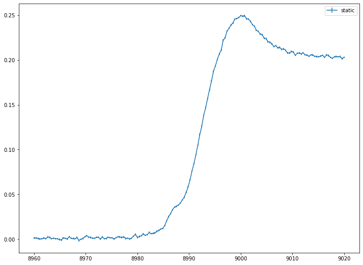
# Generates fake experiment data
# Model: sum of 3 voigt profile and one gaussian edge fature

e0_1 = 8987
e0_2 = 9000
e0_edge = 8992
fwhm_G_1 = 0.8
fwhm_G_2 = 0.9
fwhm_L_1 = 3
fwhm_L_2 = 9
fwhm_edge = 7

# set scan range
e = np.linspace(8960, 9020, 160)

# generate model spectrum
model_static = 0.1*voigt(e-e0_1, fwhm_G_1, fwhm_L_1) + \
    0.7*voigt(e-e0_2, fwhm_G_2, fwhm_L_2) + \
        0.2*edge_gaussian(e-e0_edge, fwhm_edge)

# set noise level
eps = 1/1000
# generate random noise
noise_static = np.random.normal(0, eps, model_static.size)

# generate measured static spectrum
obs_static = model_static + noise_static
eps_static = eps*np.ones_like(model_static)
# plot model experimental data

plt.errorbar(e, obs_static, eps_static, label='static')
plt.legend()
plt.show()
# import needed module for fitting
from TRXASprefitpack import fit_static_voigt

# set initial guess
e0_init = np.array([9000]) # initial peak position
fwhm_G_init = np.array([0]) # fwhm_G = 0 -> lorenzian
fwhm_L_init = np.array([8])

e0_edge = np.array([8995]) # initial edge position
fwhm_edge = np.array([15]) # initial edge width

fit_result_static = fit_static_voigt(e0_init, fwhm_G_init, fwhm_L_init, edge='g', edge_pos_init=e0_edge,
 edge_fwhm_init = fwhm_edge, do_glb=True, e=e, intensity=obs_static, eps=eps_static)
# print fitting result
print(fit_result_static)
[Model information]
    model : voigt
    edge: g

[Optimization Method]
    global: basinhopping
    leastsq: trf

[Optimization Status]
    nfev: 1639
    status: 0
    global_opt msg: requested number of basinhopping iterations completed successfully
    leastsq_opt msg: `xtol` termination condition is satisfied.

[Optimization Results]
    Data points: 160
    Number of effective parameters: 6
    Degree of Freedom: 154
    Chi squared:  897.505
    Reduced chi squared:  5.828
    AIC (Akaike Information Criterion statistic):  287.9112
    BIC (Bayesian Information Criterion statistic):  306.3622

[Parameters]
    e0_1:  8998.88484487 +/-  0.14751224 ( 0.00%)
    fwhm_(G, 1):  0.00000000 +/-  0.00000000 ( 0.00%)
    fwhm_(L, 1):  10.94428785 +/-  0.34837526 ( 3.18%)
    E0_(g, 1):  8992.32311424 +/-  0.08069992 ( 0.00%)
    fwhm_(G, edge, 1):  8.84961783 +/-  0.14689554 ( 1.66%)

[Parameter Bound]
    e0_1:  8996 <=  8998.88484487 <=  9004
    fwhm_(G, 1):  0 <=  0.00000000 <=  0
    fwhm_(L, 1):  4 <=  10.94428785 <=  16
    E0_(g, 1):  8965 <=  8992.32311424 <=  9025
    fwhm_(G, edge, 1):  7.5 <=  8.84961783 <=  30

[Component Contribution]
    Static spectrum
     voigt 1:  83.05%
     g type edge 1:  16.95%

[Parameter Correlation]
    Parameter Correlations >  0.1 are reported.
    (fwhm_(L, 1), e0_1) = -0.224
    (E0_(g, 1), e0_1) = -0.839
    (E0_(g, 1), fwhm_(L, 1)) =  0.479
    (fwhm_(G, edge, 1), e0_1) = -0.537
    (fwhm_(G, edge, 1), fwhm_(L, 1)) = -0.294
    (fwhm_(G, edge, 1), E0_(g, 1)) =  0.44
Using static_spectrum function in TRXASprefitpack, you can directly evaluates fitted static spectrum from fitting result
# plot fitting result and experimental data
from TRXASprefitpack import static_spectrum

plt.errorbar(e, obs_static, eps_static, label=f'expt', color='black')
plt.errorbar(e, static_spectrum(e, fit_result_static), label=f'fit', color='red')

plt.legend()
plt.show()
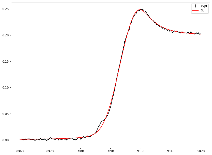
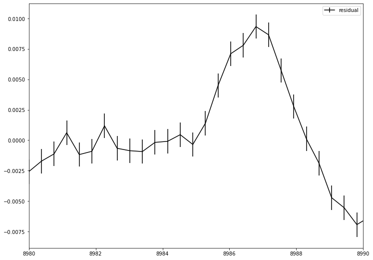
There exists one more peak near 8985 eV Region. To check this peak feature plot residual.
# plot residual

plt.errorbar(e, obs_static-static_spectrum(e, fit_result_static), eps_static, label=f'residual', color='black')

plt.legend()
plt.xlim(8980, 8990)
plt.show()
# try with two voigt feature
# set initial guess from previous fitting result and
# current observation

# set initial guess
e0_init = np.array([8987, 8999]) # initial peak position
fwhm_G_init = np.array([0, 0]) # fwhm_G = 0 -> lorenzian
fwhm_L_init = np.array([3, 11])

e0_edge = np.array([8992.3]) # initial edge position
fwhm_edge = np.array([9]) # initial edge width

fit_result_static_2 = fit_static_voigt(e0_init, fwhm_G_init, fwhm_L_init, edge='g', edge_pos_init=e0_edge,
 edge_fwhm_init = fwhm_edge, do_glb=True, e=e, intensity=obs_static, eps=eps_static)
# print fitting result
print(fit_result_static_2)
[Model information]
    model : voigt
    edge: g

[Optimization Method]
    global: basinhopping
    leastsq: trf

[Optimization Status]
    nfev: 2348
    status: 0
    global_opt msg: requested number of basinhopping iterations completed successfully
    leastsq_opt msg: `xtol` termination condition is satisfied.

[Optimization Results]
    Data points: 160
    Number of effective parameters: 9
    Degree of Freedom: 151
    Chi squared:  168.0966
    Reduced chi squared:  1.1132
    AIC (Akaike Information Criterion statistic):  25.8984
    BIC (Bayesian Information Criterion statistic):  53.575

[Parameters]
    e0_1:  8986.99315097 +/-  0.05971437 ( 0.00%)
    e0_2:  9000.00117106 +/-  0.05194541 ( 0.00%)
    fwhm_(G, 1):  0.00000000 +/-  0.00000000 ( 0.00%)
    fwhm_(G, 2):  0.00000000 +/-  0.00000000 ( 0.00%)
    fwhm_(L, 1):  3.30000708 +/-  0.18502676 ( 5.61%)
    fwhm_(L, 2):  8.85570264 +/-  0.18379219 ( 2.08%)
    E0_(g, 1):  8992.01083058 +/-  0.01895717 ( 0.00%)
    fwhm_(G, edge, 1):  6.99740613 +/-  0.08094771 ( 1.16%)

[Parameter Bound]
    e0_1:  8985.5 <=  8986.99315097 <=  8988.5
    e0_2:  8993.5 <=  9000.00117106 <=  9004.5
    fwhm_(G, 1):  0 <=  0.00000000 <=  0
    fwhm_(G, 2):  0 <=  0.00000000 <=  0
    fwhm_(L, 1):  1.5 <=  3.30000708 <=  6
    fwhm_(L, 2):  5.5 <=  8.85570264 <=  22
    E0_(g, 1):  8974.3 <=  8992.01083058 <=  9010.3
    fwhm_(G, edge, 1):  4.5 <=  6.99740613 <=  18

[Component Contribution]
    Static spectrum
     voigt 1:  10.56%
     voigt 2:  69.27%
     g type edge 1:  20.17%

[Parameter Correlation]
    Parameter Correlations >  0.1 are reported.
    (e0_2, e0_1) =  0.28
    (fwhm_(L, 1), e0_1) =  0.405
    (fwhm_(L, 1), e0_2) =  0.366
    (fwhm_(L, 2), e0_1) = -0.187
    (fwhm_(L, 2), e0_2) = -0.51
    (fwhm_(L, 2), fwhm_(L, 1)) = -0.406
    (E0_(g, 1), e0_1) =  0.275
    (E0_(g, 1), e0_2) = -0.423
    (E0_(g, 1), fwhm_(L, 1)) =  0.192
    (E0_(g, 1), fwhm_(L, 2)) =  0.48
    (fwhm_(G, edge, 1), e0_1) = -0.53
    (fwhm_(G, edge, 1), e0_2) = -0.696
    (fwhm_(G, edge, 1), fwhm_(L, 1)) = -0.556
    (fwhm_(G, edge, 1), fwhm_(L, 2)) =  0.533
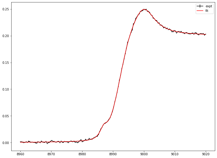
# plot fitting result and experimental data

plt.errorbar(e, obs_static, eps_static, label=f'expt', color='black')
plt.errorbar(e, static_spectrum(e, fit_result_static_2), label=f'fit', color='red')

plt.legend()
plt.show()
# save and load fitting result
from TRXASprefitpack import save_StaticResult, load_StaticResult

save_StaticResult(fit_result_static_2, 'static_example_voigt') # save fitting result to static_example_voigt.h5
loaded_result = load_StaticResult('static_example_voigt') # load fitting result from static_example_voigt.h5
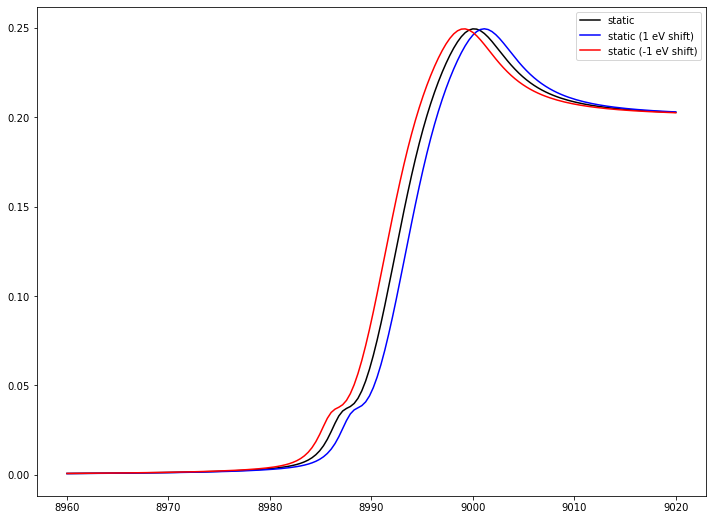
# plot static spectrum
plt.plot(e, static_spectrum(e, loaded_result), label='static', color='black')
plt.plot(e, static_spectrum(e-1, loaded_result), label='static (1 eV shift)', color='blue')
plt.plot(e, static_spectrum(e+1, loaded_result), label='static (-1 eV shift)', color='red')
plt.legend()
plt.show()
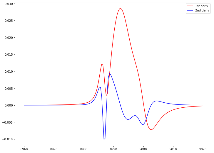
# plot its derivative up to second
plt.plot(e, static_spectrum(e, loaded_result, deriv_order=1), label='1st deriv', color='red')
plt.plot(e, static_spectrum(e, loaded_result, deriv_order=2), label='2nd deriv', color='blue')
plt.legend()
plt.show()
Optionally, you can calculated F-test based confidence interval
from TRXASprefitpack import confidence_interval

ci_result = confidence_interval(loaded_result, 0.05) # set significant level: 0.05 -> 95% confidence level
print(ci_result) # report confidence interval
[Report for Confidence Interval]
    Method: f
    Significance level:  5.000000e-02

[Confidence interval]
    8986.99315097 -  0.11770107 <= b'e0_1' <=  8986.99315097 +  0.12221621
    9000.00117106 -  0.10657343 <= b'e0_2' <=  9000.00117106 +  0.09992437
    3.30000708 -  0.35298444 <= b'fwhm_(L, 1)' <=  3.30000708 +  0.37578051
    8.85570264 -  0.34768767 <= b'fwhm_(L, 2)' <=  8.85570264 +  0.36370862
    8992.01083058 -  0.03687848 <= b'E0_(g, 1)' <=  8992.01083058 +  0.03795574
    6.99740613 -  0.15757552 <= b'fwhm_(G, edge, 1)' <=  6.99740613 +  0.162833
# compare with ase
from scipy.stats import norm

factor = norm.ppf(1-0.05/2)

print('[Confidence interval (from ASE)]')
for i in range(loaded_result['param_name'].size):
    print(f"{loaded_result['x'][i] :.8f} - {factor*loaded_result['x_eps'][i] :.8f}",
          f"<= {loaded_result['param_name'][i]} <=", f"{loaded_result['x'][i] :.8f} + {factor*loaded_result['x_eps'][i] :.8f}")
[Confidence interval (from ASE)]
8986.99315097 - 0.11703801 <= b'e0_1' <= 8986.99315097 + 0.11703801
9000.00117106 - 0.10181114 <= b'e0_2' <= 9000.00117106 + 0.10181114
0.00000000 - 0.00000000 <= b'fwhm_(G, 1)' <= 0.00000000 + 0.00000000
0.00000000 - 0.00000000 <= b'fwhm_(G, 2)' <= 0.00000000 + 0.00000000
3.30000708 - 0.36264579 <= b'fwhm_(L, 1)' <= 3.30000708 + 0.36264579
8.85570264 - 0.36022606 <= b'fwhm_(L, 2)' <= 8.85570264 + 0.36022606
8992.01083058 - 0.03715536 <= b'E0_(g, 1)' <= 8992.01083058 + 0.03715536
6.99740613 - 0.15865460 <= b'fwhm_(G, edge, 1)' <= 6.99740613 + 0.15865460
In many case, ASE does not much different from more sophisticated f-test based error estimation.