fit_static Basic Example
Basic usage example fit_static utility.
Yon can find example file from TRXASprefitpack-example fit_static subdirectory.
Fitting with voigt profile
Go to
voigtsub-directory. Invoigtsub directory, you can findexample_static_voigt.txtfile. This example is generated from Library example, fitting with static spectrum (model: voigt).Type
fit_static -hThen it prints help message. You can find detailed description of arguments in the utility section of this document.First find edge feature. Type
fit_static example_static.txt --mode voigt --edge g --e0_edge 8992 --fwhm_edge 10 -o edge --method_glb ampgo.
The first and the only one positional argument is the filename of static spectrum file to read.
Second optional argument --mode sets fitting model, we set --mode voigt that is fitting with sum of voigt component.
Third optional argument --edge, if it is not set, it does not include edge feature. In this example we set --edge g, that is gaussian type edge.
Fourth optional argument --e0_edge is initial edge position.
Fifth optional argument is --fwhm_edge initial guess for fwhm paramter of edge.
Last optional argument is -o it sets name of hdf5 file to save fitting result and directory to save text file format of fitting result.
After fitting process is finished, you can see both fitting result plot and report for fitting result in the console. Upper part of plot shows fitting curve and experimental data. Lower part of plot shows residual of fit (data-fit).
Inspecting residual panel, we can find two voigt component centered near 8985 and 9000
Based on this now add two voigt component.
Type
fit_static example_static.txt --mode voigt --e0_voigt 8985 9000 --fwhm_L_voigt 2 6 --edge g --e0_edge 8992 --fwhm_edge 10 -o fit --method_glb ampgo.
First additional optional argument --e0_voigt sets initial peak position of voigt component
Second additional optional argument --fwhm_L_voigt sets initial fwhm parameter of voigt component. In this example we only set lorenzian part of voigt componnet, so our voigt component is indeed lorenzian component.
After fitting process is finished, you can see fitting result plot.
Description for Output file in fit directory.
fit.txtcontains fitting and each component curveweight.txtweight of each fitting componentfit_summary.txtSummary of fitting result.res.txtcontains residual of fit
Fitting with theoretical calculated line spectrum
Go to
thysub-directory. Inthysub directory, you can findexample_static_thy.txtfile. This example is generated from Library example, fitting with static spectrum (model: thy).
Check thoeretical Spectrum
Type
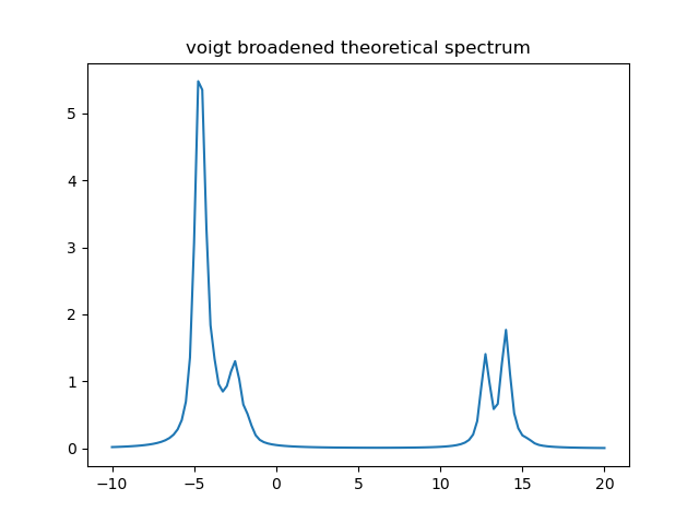
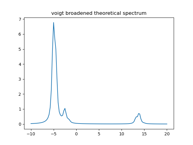
calc_broad Ni_example_1.stk -10 20 0.25 0.3 0.5 --policy scale --peak_shift 0 -o Ni_tst_1Then
calc_broadcalculates voigt broadened thoeretical spectrum with fwhm_G 0.3 and fwhm_L 0.5 from -10 to 20 with 0.25 step.Type
calc_broad Ni_example_2.stk -10 20 0.25 0.3 0.5 --policy scale --peak_shift 0 -o Ni_tst_2Then
calc_broaddo the samething withNi_example_2.stkfile.
Ni_example_1
Ni_example_2
fitting with theoretical Spectrum
First try with one theoretical Spectrum
Type
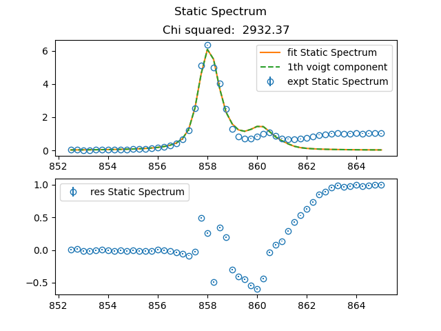
fit_static example_static_thy.txt --mode thy --thy_file Ni_example_1.stk --fwhm_G_thy 0.3 --fwhm_L_thy 0.5 --policy shift --peak_shift 863 -o fit_thy_1 --method_glb ampgo.
In this command, you set --mode thy and --thy_file Ni_example_1.stk, so you use fitting static spectrum with voigt broadened thoeretical line shape spectrum and it reads thoretical peak position and intensity from Ni_example_1.stk.
Moreover, you set uniform fwhm paramter for such voigt function through --fwhm_G_thy and --fwhm_L_thy option.
To resolve discrepency between thoretical peak position and peak position of static spectrum, you can set --policy. In this example you set --policy shift. So, it shift peak position of thoretical spectrum to match peak position. To do this you should set initial peak shift paramter via --peak_shift option. We set initial peak shift paramter to 863 (--peak_shift 863).
fit_thy_1
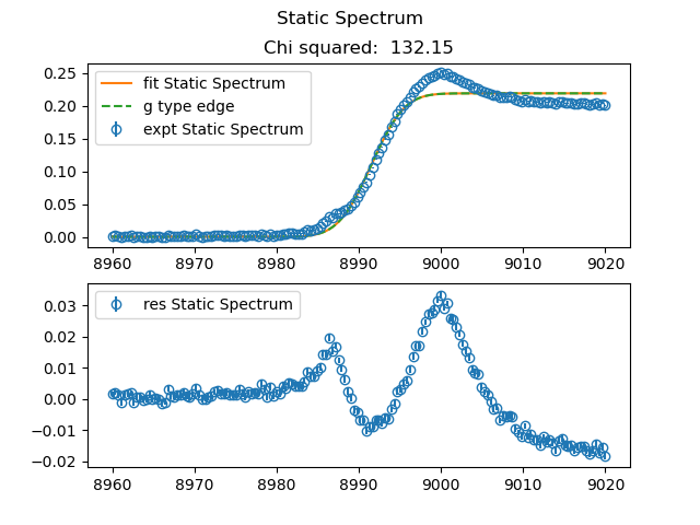
Next try with two theoretical Spectrum
Type
fit_static example_static_thy.txt --mode thy --thy_file Ni_example_1.stk Ni_example_2.stk --fwhm_G_thy 0.3 --fwhm_L_thy 0.5 --policy shift --peak_shift 863 863 -o fit_thy_2 --method_glb ampgo.
fit_thy_2
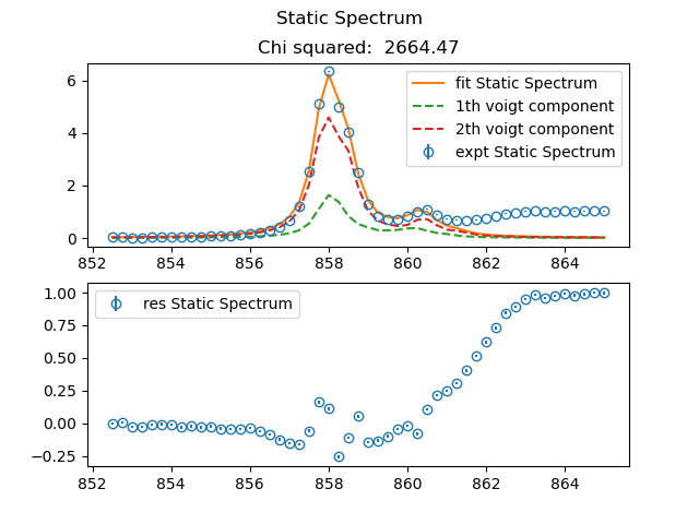
Look at the residual pannel, then you find gaussian type edge feature which is centered at 862 and its fwhm is about 2.
Now add one gaussian type edge feature. Before adding one edge feature, you should refine your initial guess based on previous fitting result.
Type
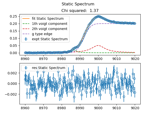
fit_static example_static_thy.txt --mode thy --thy_file Ni_example_1.stk Ni_example_2.stk --fwhm_G_thy 0.3 --fwhm_L_thy 0.5 --policy shift --peak_shift 862.5 863 --edge g --fwhm_edge 2 --e0_edge 862 -o fit_thy_2_edge_1 --method_glb ampgo.
fit_thy_2_edge_1
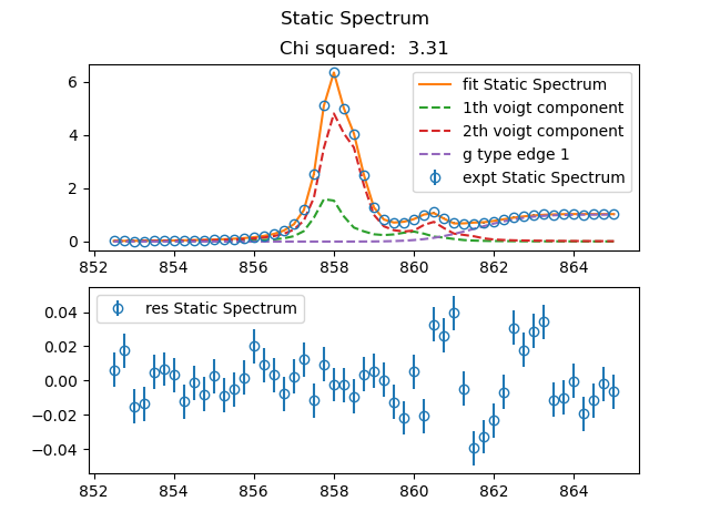
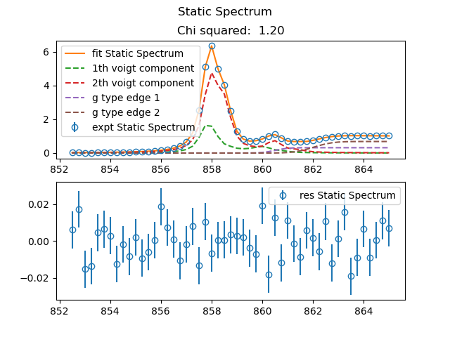
Add one more gaussian type edge feature.
Type
fit_static example_static_thy.txt --mode thy --thy_file Ni_example_1.stk Ni_example_2.stk --fwhm_G_thy 0.3 --fwhm_L_thy 0.5 --policy shift --peak_shift 862.5 863 --edge g --fwhm_edge 1 2 --e0_edge 860.5 862 -o fit_thy_2_edge_2 --method_glb ampgo.
fit_thy_2_edge_2