Fitting with Static spectrum (Model: theoretical spectrum)
Objective
Fitting with voigt broadened theoretical spectrum
Save and Load fitting result
Retrieve or interpolate experimental spectrum based on fitting result and calculates its derivative up to 2.
# import needed module
import numpy as np
import matplotlib.pyplot as plt
import TRXASprefitpack
from TRXASprefitpack import voigt_thy, edge_gaussian
plt.rcParams["figure.figsize"] = (12,9)
Version information
print(TRXASprefitpack.__version__)
0.6.1
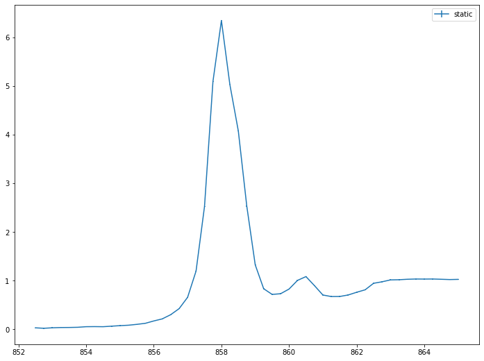
# Generates fake experiment data
# Model: sum of 2 normalized theoretical spectrum

edge_type = 'g'
e0_edge = np.array([860.5, 862])
fwhm_edge = np.array([1, 1.5])
peak_shift = np.array([862.5, 863])
mixing = np.array([0.3, 0.7])
mixing_edge = np.array([0.3, 0.7])
fwhm_G_thy = 0.3
fwhm_L_thy = 0.5

thy_peak = np.empty(2, dtype=object)
thy_peak[0] = np.genfromtxt('Ni_example_1.stk')
thy_peak[1] = np.genfromtxt('Ni_example_2.stk')

# set scan range
e = np.linspace(852.5, 865, 51)

# generate model spectrum
model_static = mixing[0]*voigt_thy(e, thy_peak[0], fwhm_G_thy, fwhm_L_thy,
peak_shift[0], policy='shift')+\
    mixing[1]*voigt_thy(e, thy_peak[1], fwhm_G_thy, fwhm_L_thy,
    peak_shift[1], policy='shift')+\
        mixing_edge[0]*edge_gaussian(e-e0_edge[0], fwhm_edge[0])+\
            mixing_edge[1]*edge_gaussian(e-e0_edge[1], fwhm_edge[1])

# set noise level
eps = 1/100
# generate random noise
noise_static = np.random.normal(0, eps, model_static.size)

# generate measured static spectrum
obs_static = model_static + noise_static
eps_static = eps*np.ones_like(model_static)
# plot model experimental data

plt.errorbar(e, obs_static, eps_static, label='static')
plt.legend()
plt.show()
Before fitting, we need to guess about initial peak shift paramter for theoretical spectrum
# Guess initial peak_shift
# check with arbitary fwhm paramter and peak_shift paramter
e_tst = np.linspace(-10, 20, 120)
comp_1 = voigt_thy(e_tst, thy_peak[0], 0.5, 1, 0, policy='shift')
comp_2 = voigt_thy(e_tst, thy_peak[1], 0.5, 1, 0, policy='shift')

plt.plot(e_tst, comp_1, label='comp_1')
plt.plot(e_tst, comp_2, label='comp_2')
plt.legend()
plt.show()
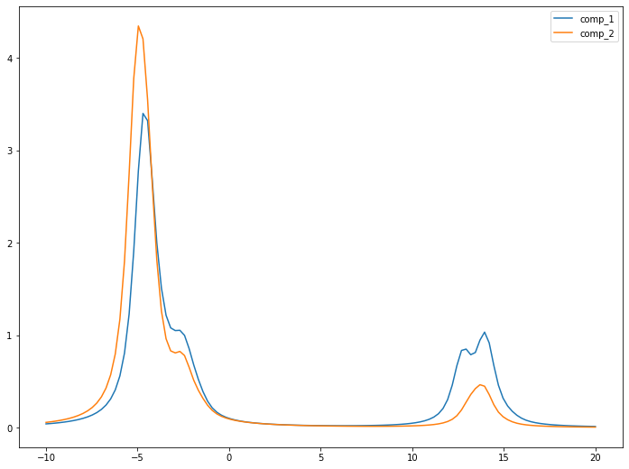
Compare first peak position, we can set initial peak shift paramter for both component as \(863\), \(863\). First try with only one component
from TRXASprefitpack import fit_static_thy
# initial guess
policy = 'shift'
peak_shift_init = np.array([863])
fwhm_G_thy_init = 0.5
fwhm_L_thy_init = 0.5

result_1 = fit_static_thy(thy_peak[:1], fwhm_G_thy_init, fwhm_L_thy_init, policy, peak_shift_init, do_glb=True,
e=e, intensity=obs_static, eps=eps_static)
print(result_1)
[Model information]
    model : thy
    policy: shift

[Optimization Method]
    global: basinhopping
    leastsq: trf

[Optimization Status]
    nfev: 1596
    status: 0
    global_opt msg: requested number of basinhopping iterations completed successfully
    leastsq_opt msg: `xtol` termination condition is satisfied.

[Optimization Results]
    Data points: 51
    Number of effective parameters: 4
    Degree of Freedom: 47
    Chi squared:  137613.5102
    Reduced chi squared:  2927.947
    AIC (Akaike Information Criterion statistic):  410.9193
    BIC (Bayesian Information Criterion statistic):  418.6466

[Parameters]
    fwhm_G:  0.52544619 +/-  0.31400904 ( 59.76%)
    fwhm_L:  0.54033663 +/-  0.23813406 ( 44.07%)
    peak_shift 1:  862.66542093 +/-  0.03396275 ( 0.00%)

[Parameter Bound]
    fwhm_G:  0.25 <=  0.52544619 <=  1
    fwhm_L:  0.25 <=  0.54033663 <=  1
    peak_shift 1:  862.59060102 <=  862.66542093 <=  863.40939898

[Component Contribution]
    Static spectrum
     thy 1:  100.00%

[Parameter Correlation]
    Parameter Correlations >  0.1 are reported.
    (fwhm_L, fwhm_G) = -0.919
Using static_spectrum function in TRXASprefitpack, you can directly evaluates fitted static spectrum from fitting result
# plot fitting result and experimental data
from TRXASprefitpack import static_spectrum

plt.errorbar(e, obs_static, eps_static, label=f'expt', color='black')
plt.errorbar(e, static_spectrum(e, result_1), label=f'fit', color='red')

plt.legend()
plt.show()
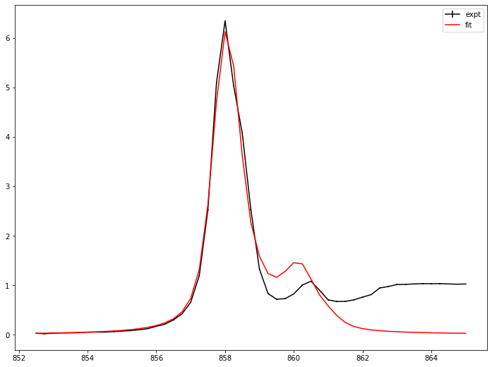
The fit looks not good, there may exists one more component.
# initial guess
# add one more thoeretical spectrum
policy = 'shift'
peak_shift_init = np.array([863, 863])
# Note that each thoeretical spectrum shares full width at half maximum paramter
fwhm_G_thy_init = 0.5
fwhm_L_thy_init = 0.5

result_2 = fit_static_thy(thy_peak, fwhm_G_thy_init, fwhm_L_thy_init, policy, peak_shift_init, do_glb=True,
e=e, intensity=obs_static, eps=eps_static)
print(result_2)
[Model information]
    model : thy
    policy: shift

[Optimization Method]
    global: basinhopping
    leastsq: trf

[Optimization Status]
    nfev: 2246
    status: 0
    global_opt msg: requested number of basinhopping iterations completed successfully
    leastsq_opt msg: Both `ftol` and `xtol` termination conditions are satisfied.

[Optimization Results]
    Data points: 51
    Number of effective parameters: 6
    Degree of Freedom: 45
    Chi squared:  119985.2676
    Reduced chi squared:  2666.3393
    AIC (Akaike Information Criterion statistic):  407.9282
    BIC (Bayesian Information Criterion statistic):  419.5192

[Parameters]
    fwhm_G:  0.25000000 +/-  0.44683487 ( 178.73%)
    fwhm_L:  0.60579241 +/-  0.20775859 ( 34.30%)
    peak_shift 1:  862.59060102 +/-  0.24407807 ( 0.03%)
    peak_shift 2:  862.98069401 +/-  0.11409659 ( 0.01%)

[Parameter Bound]
    fwhm_G:  0.25 <=  0.25000000 <=  1
    fwhm_L:  0.25 <=  0.60579241 <=  1
    peak_shift 1:  862.59060102 <=  862.59060102 <=  863.40939898
    peak_shift 2:  862.59060102 <=  862.98069401 <=  863.40939898

[Component Contribution]
    Static spectrum
     thy 1:  32.73%
     thy 2:  67.27%

[Parameter Correlation]
    Parameter Correlations >  0.1 are reported.
    (fwhm_L, fwhm_G) = -0.885
    (peak_shift 1, fwhm_G) = -0.35
    (peak_shift 1, fwhm_L) =  0.491
    (peak_shift 2, fwhm_G) =  0.436
    (peak_shift 2, fwhm_L) = -0.543
    (peak_shift 2, peak_shift 1) = -0.856
plt.errorbar(e, obs_static, eps_static, label=f'expt', color='black')
plt.errorbar(e, static_spectrum(e, result_2), label=f'fit', color='red')

plt.legend()
plt.show()
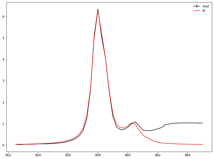
# plot residual
plt.errorbar(e, obs_static-static_spectrum(e, result_2), eps_static, label=f'res', color='red')

plt.legend()
plt.show()
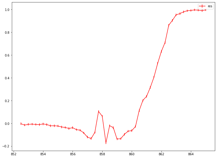
Residual suggests that there exists gaussian edge feature near 862 with fwhm 2
# try with two theoretical component and edge

# refine initial guess
policy = 'shift'
peak_shift_init = np.array([862.6, 863])
# Note that each thoeretical spectrum shares full width at half maximum paramter
fwhm_G_thy_init = 0.25
fwhm_L_thy_init = 0.5
# add one edge feature
e0_edge_init = np.array([862])
fwhm_edge_init = np.array([2])

result_2_edge = fit_static_thy(thy_peak, fwhm_G_thy_init, fwhm_L_thy_init, policy, peak_shift_init,
edge='g', edge_pos_init=e0_edge_init, edge_fwhm_init=fwhm_edge_init, do_glb=True,
e=e, intensity=obs_static, eps=eps_static)
# print fitting result
print(result_2_edge)
[Model information]
    model : thy
    policy: shift
    edge: g

[Optimization Method]
    global: basinhopping
    leastsq: trf

[Optimization Status]
    nfev: 3767
    status: 0
    global_opt msg: requested number of basinhopping iterations completed successfully
    leastsq_opt msg: `xtol` termination condition is satisfied.

[Optimization Results]
    Data points: 51
    Number of effective parameters: 9
    Degree of Freedom: 42
    Chi squared:  110.5689
    Reduced chi squared:  2.6326
    AIC (Akaike Information Criterion statistic):  57.4645
    BIC (Bayesian Information Criterion statistic):  74.8509

[Parameters]
    fwhm_G:  0.30072514 +/-  0.00955020 ( 3.18%)
    fwhm_L:  0.50194070 +/-  0.00710896 ( 1.42%)
    peak_shift 1:  862.49916688 +/-  0.00784966 ( 0.00%)
    peak_shift 2:  862.99880820 +/-  0.00335302 ( 0.00%)
    E0_g 1:  861.58985863 +/-  0.01883188 ( 0.00%)
    fwhm_(g, edge 1):  2.27083148 +/-  0.06169109 ( 2.72%)

[Parameter Bound]
    fwhm_G:  0.125 <=  0.30072514 <=  0.5
    fwhm_L:  0.25 <=  0.50194070 <=  1
    peak_shift 1:  862.29557969 <=  862.49916688 <=  862.90442031
    peak_shift 2:  862.69557969 <=  862.99880820 <=  863.30442031
    E0_g 1:  858 <=  861.58985863 <=  866
    fwhm_(g, edge 1):  1 <=  2.27083148 <=  4

[Component Contribution]
    Static spectrum
     thy 1:  14.25%
     thy 2:  35.45%
     g type edge 1:  50.30%

[Parameter Correlation]
    Parameter Correlations >  0.1 are reported.
    (fwhm_L, fwhm_G) = -0.838
    (peak_shift 1, fwhm_G) = -0.287
    (peak_shift 1, fwhm_L) =  0.599
    (peak_shift 2, fwhm_G) =  0.371
    (peak_shift 2, fwhm_L) = -0.609
    (peak_shift 2, peak_shift 1) = -0.66
    (E0_g 1, fwhm_G) = -0.144
    (E0_g 1, fwhm_L) =  0.193
    (E0_g 1, peak_shift 1) =  0.137
    (fwhm_(g, edge 1), fwhm_G) =  0.109
    (fwhm_(g, edge 1), fwhm_L) = -0.171
    (fwhm_(g, edge 1), peak_shift 1) = -0.184
    (fwhm_(g, edge 1), E0_g 1) =  0.206
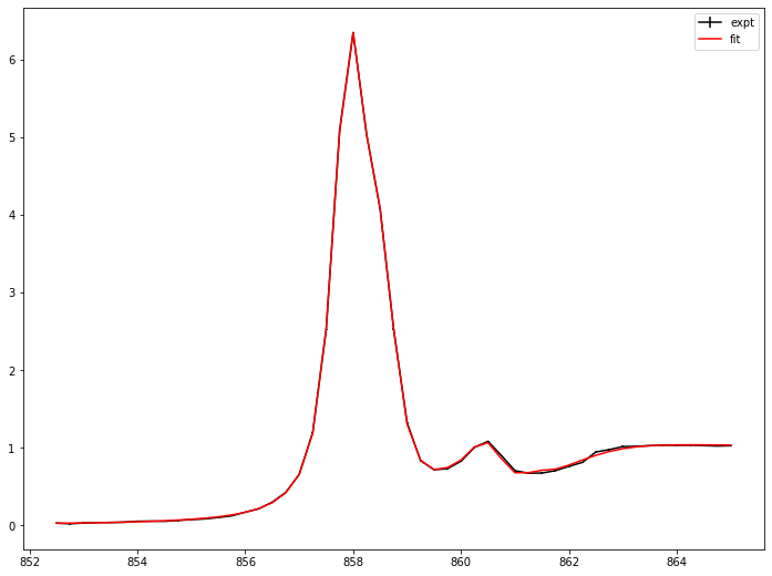
# plot fitting result and experimental data

plt.errorbar(e, obs_static, eps_static, label=f'expt', color='black')
plt.errorbar(e, static_spectrum(e, result_2_edge), label=f'fit', color='red')

plt.legend()
plt.show()
# plot residual
plt.errorbar(e, obs_static-static_spectrum(e, result_2_edge), eps_static, label=f'fit', color='red')

plt.legend()
plt.show()
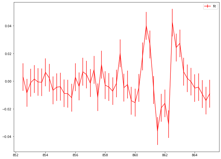
fit_static_thy supports adding multiple edge feature, to demenstrate this I add one more edge feature in the fitting model.
# add one more edge

# refine initial guess
policy = 'shift'
peak_shift_init = np.array([862.6, 863])
# Note that each thoeretical spectrum shares full width at half maximum paramter
fwhm_G_thy_init = 0.25
fwhm_L_thy_init = 0.5
# add one edge feature
e0_edge_init = np.array([860.5, 862])
fwhm_edge_init = np.array([0.8, 1.5])

result_2_edge_2 = fit_static_thy(thy_peak, fwhm_G_thy_init, fwhm_L_thy_init, policy, peak_shift_init,
edge='g', edge_pos_init=e0_edge_init, edge_fwhm_init=fwhm_edge_init, do_glb=True,
e=e, intensity=obs_static, eps=eps_static)
print(result_2_edge_2)
[Model information]
    model : thy
    policy: shift
    edge: g

[Optimization Method]
    global: basinhopping
    leastsq: trf

[Optimization Status]
    nfev: 8320
    status: 0
    global_opt msg: requested number of basinhopping iterations completed successfully
    leastsq_opt msg: `xtol` termination condition is satisfied.

[Optimization Results]
    Data points: 51
    Number of effective parameters: 12
    Degree of Freedom: 39
    Chi squared:  34.0751
    Reduced chi squared:  0.8737
    AIC (Akaike Information Criterion statistic):  3.4338
    BIC (Bayesian Information Criterion statistic):  26.6158

[Parameters]
    fwhm_G:  0.29705630 +/-  0.00561125 ( 1.89%)
    fwhm_L:  0.50587743 +/-  0.00416873 ( 0.82%)
    peak_shift 1:  862.50271730 +/-  0.00468196 ( 0.00%)
    peak_shift 2:  862.99964539 +/-  0.00195884 ( 0.00%)
    E0_g 1:  861.95968431 +/-  0.04259326 ( 0.00%)
    E0_g 2:  860.47220697 +/-  0.05153850 ( 0.01%)
    fwhm_(g, edge 1):  1.50379841 +/-  0.08769146 ( 5.83%)
    fwhm_(g, edge 2):  0.82825820 +/-  0.12320940 ( 14.88%)

[Parameter Bound]
    fwhm_G:  0.125 <=  0.29705630 <=  0.5
    fwhm_L:  0.25 <=  0.50587743 <=  1
    peak_shift 1:  862.29557969 <=  862.50271730 <=  862.90442031
    peak_shift 2:  862.69557969 <=  862.99964539 <=  863.30442031
    E0_g 1:  858.9 <=  861.95968431 <=  862.1
    E0_g 2:  859 <=  860.47220697 <=  865
    fwhm_(g, edge 1):  0.4 <=  1.50379841 <=  1.6
    fwhm_(g, edge 2):  0.75 <=  0.82825820 <=  3

[Component Contribution]
    Static spectrum
     thy 1:  14.79%
     thy 2:  35.30%
     g type edge 1:  36.63%
     g type edge 2:  13.28%

[Parameter Correlation]
    Parameter Correlations >  0.1 are reported.
    (fwhm_L, fwhm_G) = -0.84
    (peak_shift 1, fwhm_G) = -0.313
    (peak_shift 1, fwhm_L) =  0.624
    (peak_shift 2, fwhm_G) =  0.388
    (peak_shift 2, fwhm_L) = -0.624
    (peak_shift 2, peak_shift 1) = -0.665
    (E0_g 1, peak_shift 1) = -0.142
    (E0_g 2, E0_g 1) =  0.866
    (fwhm_(g, edge 1), peak_shift 1) =  0.114
    (fwhm_(g, edge 1), E0_g 1) = -0.853
    (fwhm_(g, edge 1), E0_g 2) = -0.757
    (fwhm_(g, edge 2), fwhm_G) =  0.126
    (fwhm_(g, edge 2), fwhm_L) = -0.226
    (fwhm_(g, edge 2), peak_shift 1) = -0.307
    (fwhm_(g, edge 2), E0_g 1) =  0.731
    (fwhm_(g, edge 2), E0_g 2) =  0.7
    (fwhm_(g, edge 2), fwhm_(g, edge 1)) = -0.602
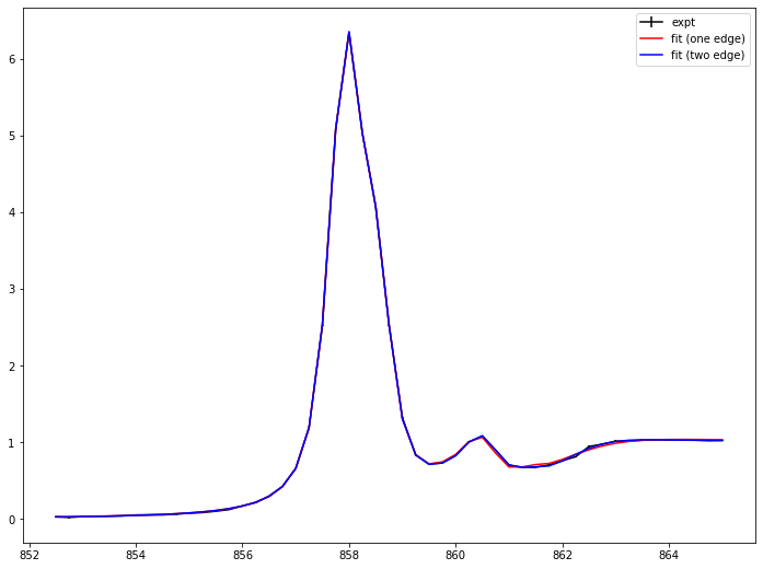
plt.errorbar(e, obs_static, eps_static, label=f'expt', color='black')
plt.errorbar(e, static_spectrum(e, result_2_edge), label=f'fit (one edge)', color='red')
plt.errorbar(e, static_spectrum(e, result_2_edge_2), label=f'fit (two edge)', color='blue')

plt.legend()
plt.show()
# save and load fitting result
from TRXASprefitpack import save_StaticResult, load_StaticResult

save_StaticResult(result_2_edge_2, 'static_example_thy') # save fitting result to static_example_thy.h5
loaded_result = load_StaticResult('static_example_thy') # load fitting result from static_example_thy.h5
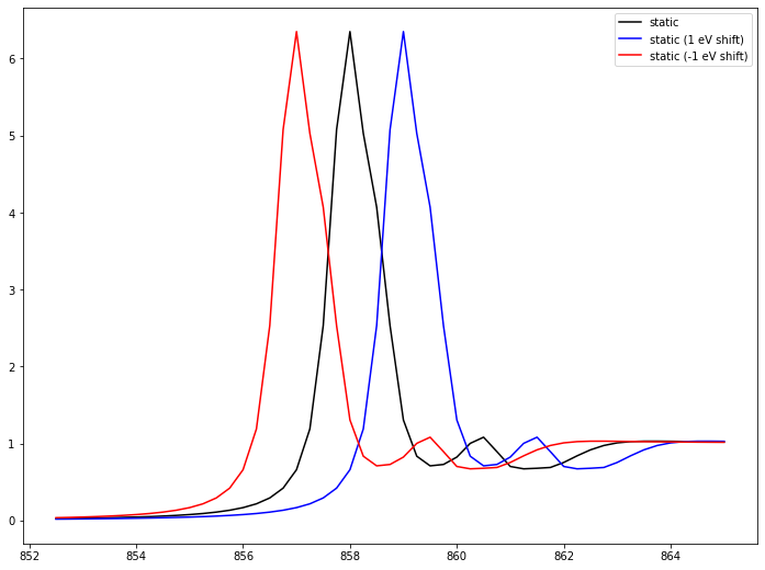
# plot static spectrum
plt.plot(e, static_spectrum(e, loaded_result), label='static', color='black')
plt.plot(e, static_spectrum(e-1, loaded_result), label='static (1 eV shift)', color='blue')
plt.plot(e, static_spectrum(e+1, loaded_result), label='static (-1 eV shift)', color='red')
plt.legend()
plt.show()
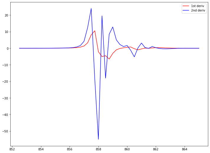
# plot its derivative up to second
plt.plot(e, static_spectrum(e, loaded_result, deriv_order=1), label='1st deriv', color='red')
plt.plot(e, static_spectrum(e, loaded_result, deriv_order=2), label='2nd deriv', color='blue')
plt.legend()
plt.show()
Optionally, you can calculated F-test based confidence interval
from TRXASprefitpack import confidence_interval

ci_result = confidence_interval(loaded_result, 0.05) # set significant level: 0.05 -> 95% confidence level
print(ci_result) # report confidence interval
[Report for Confidence Interval]
    Method: f
    Significance level:  5.000000e-02

[Confidence interval]
    0.2970563 -  0.01151555 <= b'fwhm_G' <=  0.2970563 +  0.01122604
    0.50587743 -  0.00845537 <= b'fwhm_L' <=  0.50587743 +  0.00838732
    862.5027173 -  0.00931266 <= b'peak_shift 1' <=  862.5027173 +  0.00940234
    862.99964539 -  0.00392627 <= b'peak_shift 2' <=  862.99964539 +  0.00396055
    861.95968431 -  0.07132079 <= b'E0_g 1' <=  861.95968431 +  0.10665698
    860.47220697 -  0.09237276 <= b'E0_g 2' <=  860.47220697 +  0.14202443
    1.50379841 -  0.19350716 <= b'fwhm_(g, edge 1)' <=  1.50379841 +  0.17349489
    0.8282582 -  0.23266591 <= b'fwhm_(g, edge 2)' <=  0.8282582 +  0.3153878
# compare with ase
from scipy.stats import norm

factor = norm.ppf(1-0.05/2)

print('[Confidence interval (from ASE)]')
for i in range(loaded_result['param_name'].size):
    print(f"{loaded_result['x'][i] :.8f} - {factor*loaded_result['x_eps'][i] :.8f}",
          f"<= {loaded_result['param_name'][i]} <=", f"{loaded_result['x'][i] :.8f} + {factor*loaded_result['x_eps'][i] :.8f}")
[Confidence interval (from ASE)]
0.29705630 - 0.01099785 <= b'fwhm_G' <= 0.29705630 + 0.01099785
0.50587743 - 0.00817056 <= b'fwhm_L' <= 0.50587743 + 0.00817056
862.50271730 - 0.00917647 <= b'peak_shift 1' <= 862.50271730 + 0.00917647
862.99964539 - 0.00383925 <= b'peak_shift 2' <= 862.99964539 + 0.00383925
861.95968431 - 0.08348127 <= b'E0_g 1' <= 861.95968431 + 0.08348127
860.47220697 - 0.10101361 <= b'E0_g 2' <= 860.47220697 + 0.10101361
1.50379841 - 0.17187210 <= b'fwhm_(g, edge 1)' <= 1.50379841 + 0.17187210
0.82825820 - 0.24148600 <= b'fwhm_(g, edge 2)' <= 0.82825820 + 0.24148600
In many case, ASE does not much different from more sophisticated f-test based error estimation.