IRF
Compare three kinds of instrument response function (cauchy, gaussian, pseudo voigt or voigt).
For pseudo voigt profile \({fwhm}({fwhm}_G, {fwhm}_L)\) and \(\eta({fwhm}_G, {fwhm}_L)\) is chosen according to J. Appl. Cryst. (2000). 33, 1311-1316
import numpy as np
import matplotlib.pyplot as plt
import TRXASprefitpack
from TRXASprefitpack import gau_irf, cauchy_irf, pvoigt_irf
from TRXASprefitpack import calc_eta, calc_fwhm
from TRXASprefitpack import voigt
plt.rcParams["figure.figsize"] = (12,9)
version infromation
print(TRXASprefitpack.__version__)
0.6.0
Compare cauchy and gaussian IRF with same fwhm
fwhm = 0.15 # 150 fs
t = np.linspace(-1,1,200)
cauchy = cauchy_irf(t,fwhm)
gau = gau_irf(t,fwhm)
plt.plot(t, cauchy, label='cauchy irf')
plt.plot(t, gau, label='gaussian irf')
plt.legend()
plt.show()
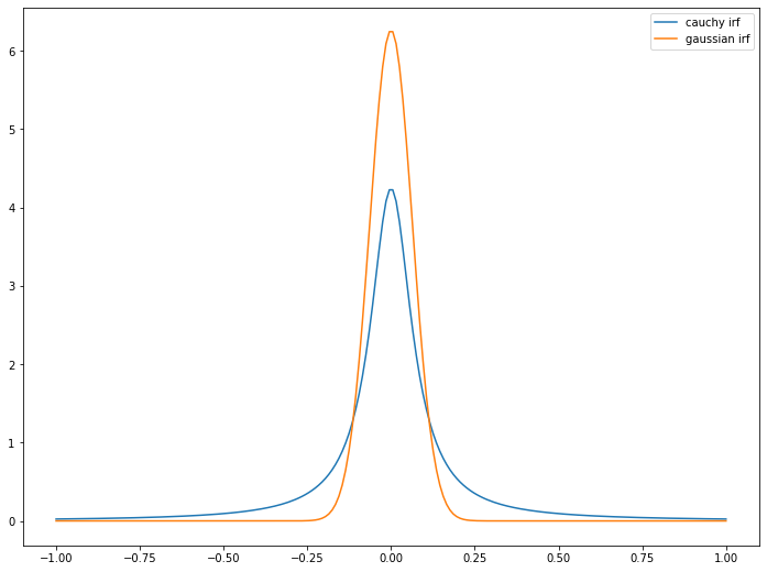
Cauchy irf is more diffuse then Gaussian irf
Compare pseudo voigt irf and voigt irf with different combination of (fwhm_G, fwhm_L)
(0.1, 0.3)
(0.1, 0.15)
(0.1, 0.1)
(0.15, 0.1)
(0.3, 0.1)
fwhm_G_1, fwhm_L_1 = (0.1, 0.3)
fwhm_G_2, fwhm_L_2 = (0.1, 0.15)
fwhm_G_3, fwhm_L_3 = (0.1, 0.1)
fwhm_G_4, fwhm_L_4 = (0.15, 0.1)
fwhm_G_5, fwhm_L_5 = (0.3, 0.1)


fwhm_1, eta_1 = (calc_fwhm(fwhm_G_1, fwhm_L_1), calc_eta(fwhm_G_1, fwhm_L_1))
fwhm_2, eta_2 = (calc_fwhm(fwhm_G_2, fwhm_L_2), calc_eta(fwhm_G_2, fwhm_L_2))
fwhm_3, eta_3 = (calc_fwhm(fwhm_G_3, fwhm_L_3), calc_eta(fwhm_G_3, fwhm_L_3))
fwhm_4, eta_4 = (calc_fwhm(fwhm_G_4, fwhm_L_4), calc_eta(fwhm_G_4, fwhm_L_4))
fwhm_5, eta_5 = (calc_fwhm(fwhm_G_5, fwhm_L_5), calc_eta(fwhm_G_5, fwhm_L_5))

pvoigt1 = pvoigt_irf(t, fwhm_1, eta_1)
pvoigt2 = pvoigt_irf(t, fwhm_2, eta_2)
pvoigt3 = pvoigt_irf(t, fwhm_3, eta_3)
pvoigt4 = pvoigt_irf(t, fwhm_4, eta_4)
pvoigt5 = pvoigt_irf(t, fwhm_5, eta_5)

voigt1 = voigt(t, fwhm_G_1, fwhm_L_1)
voigt2 = voigt(t, fwhm_G_2, fwhm_L_2)
voigt3 = voigt(t, fwhm_G_3, fwhm_L_3)
voigt4 = voigt(t, fwhm_G_4, fwhm_L_4)
voigt5 = voigt(t, fwhm_G_5, fwhm_L_5)

plt.subplot(511)
plt.plot(t, pvoigt1, label=f'pvoigt (fwhm_G, fwhm_L)=({fwhm_G_1}, {fwhm_L_1})', color='red')
plt.plot(t, voigt1, label=f'voigt (fwhm_G, fwhm_L)=({fwhm_G_1}, {fwhm_L_1})', color='blue')
plt.legend()

plt.subplot(512)
plt.plot(t, pvoigt2, label=f'pvoigt (fwhm_G, fwhm_L)=({fwhm_G_2}, {fwhm_L_2})', color='red')
plt.plot(t, voigt2, label=f'voigt (fwhm_G, fwhm_L)=({fwhm_G_2}, {fwhm_L_2})', color='blue')
plt.legend()

plt.subplot(513)
plt.plot(t, pvoigt3, label=f'pvoigt (fwhm_G, fwhm_L)=({fwhm_G_3}, {fwhm_L_3})', color='red')
plt.plot(t, voigt3, label=f'voigt (fwhm_G, fwhm_L)=({fwhm_G_3}, {fwhm_L_3})', color='blue')
plt.legend()

plt.subplot(514)
plt.plot(t, pvoigt4, label=f'pvoigt (fwhm_G, fwhm_L)=({fwhm_G_4}, {fwhm_L_4})', color='red')
plt.plot(t, voigt4, label=f'voigt (fwhm_G, fwhm_L)=({fwhm_G_4}, {fwhm_L_4})', color='blue')
plt.legend()

plt.subplot(515)
plt.plot(t, pvoigt5, label=f'pvoigt (fwhm_G, fwhm_L)=({fwhm_G_5}, {fwhm_L_5})', color='red')
plt.plot(t, voigt5, label=f'voigt (fwhm_G, fwhm_L)=({fwhm_G_5}, {fwhm_L_5})', color='blue')
plt.legend()
plt.show()
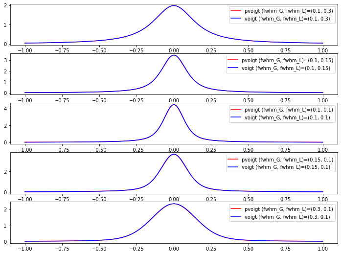
As you can see the selection of \({fwhm}\) and \(\eta\) based on J. Appl. Cryst. (2000). 33, 1311-1316 well approximates real voigt profile