fit_osc Basic Example
Basic usage example for fit_osc utility and advanced usage example for fit_tscan utility. Yon can find example file from TRXASprefitpack-example fit_osc subdirectory.
In fit_osc sub directory you can find
example_1.txt,example_2.txt,example_3.txt,example_4.txtfiles. These examples are generated from rate equation example section 2. branched decay with varying time zero of each scan around 0 ps. However lifetimes are different from rate equation section 2. brnached decay one.Type
fit_osc -hThen it prints help message. You can find detailed description of arguments in the utility section of this document.Since
fit_oscutility can not fit directly to experimental time delay scan, you should calcuate residual of experimental time delay scan fromfit_tscanorfit_sequtility. In this example we usefit_tscanutility to calculate residual of experimental time delay scan.
Calculation of residual of time delay scan
Type
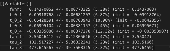
fit_tscan example --irf g --fwhm_G 0.15 -t0 0 0 0 0 --tau 3 100 500 --no_base, optionally you can turn on--slowoption to use robust global optimization methodampgoinstead of fasterNelder–Mead.After fitting process is finished, you can see both fitting result plot and report for fitting result in the console. Upper part of plot shows fitting curve and experimental data. Lower part of plot shows residual of fit (data-fit).
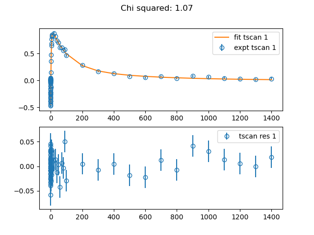
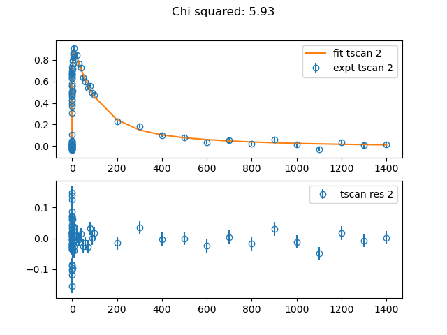
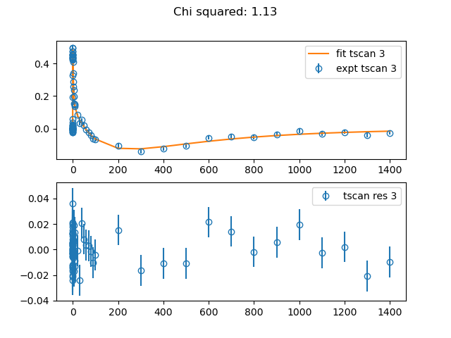
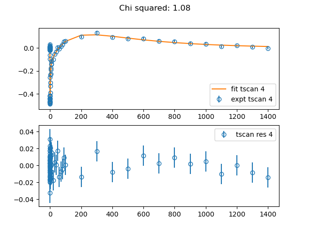
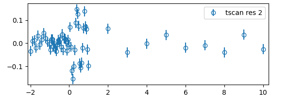
Compare chi squared and residual plot of each scan, you can find that chi squared value of tscan 2 is much higher than others and residual seems to have oscillation feature. Below plot is the residual plot of time scan 2 with time range -2 to 10.
Now close all fitting result plot windows
Fitting with residual
Note
To fitting with residual of time scan data, you should have high quality time scan.
From fitting report of previous time delay scan fitting, get full width and half maximum value of irf function and time zero of tscan 2.
Copy
example_res_2.txttoexample_osc_1.txt, since we will do residual fitting with time scan 2.Type
fit_osc -hto get help message offit_osc. Detailed descriptions would be found inutilitysection.Type
fit_osc example_osc --irf g --fwhm_G 0.14 -t0 -0.06 --tau 3 --period 0.4 --phase 0 --fix_irf. Since oscillation feature may distort time zero, we do not fix time zero value to the value from previous time scan fitting. However you can fix time zero via--fix_t0option. Optionally you can turn onampgomethod via--slowoption.After residual fitting is finished, it prints fitting result and draws plot.
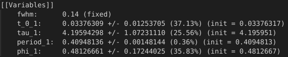
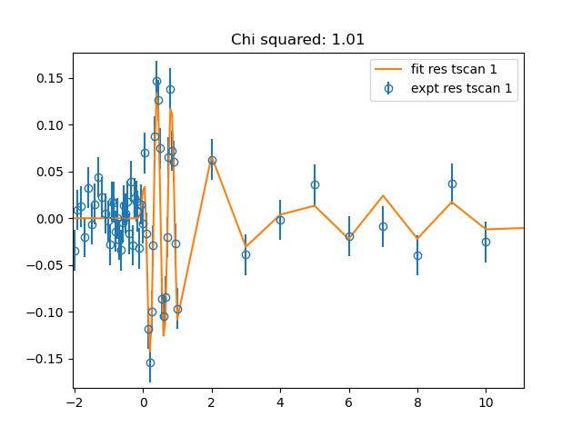
From residual fitting, we observe oscillation feature with lifetime 4 ps, vibrational period 0.4 ps or vibrational frequency 2.5 THz and phase factor \(0.5 \approx \pi/6\).