IRF
Compare three kinds of instrument response function (cauchy, gaussian, pseudo voigt)
# import needed module
import numpy as np
import matplotlib.pyplot as plt
import TRXASprefitpack
from TRXASprefitpack import gau_irf, cauchy_irf, pvoigt_irf
from TRXASprefitpack import model_n_comp_conv
plt.rcParams["figure.figsize"] = (14,10)
version infromation
print(TRXASprefitpack.__version__)
0.5.0
Define function for IRF
for pseudo voigt profile eta is chosen according to J. Appl. Cryst. (2000). 33, 1311-1316
def calc_eta(fwhm):
    f = fwhm[0]**5+2.69269*fwhm[0]**4*fwhm[1]+2.42843*fwhm[0]**3*fwhm[1]**2 + \
                    4.47163*fwhm[0]**2*fwhm[1]**3 + 0.07842*fwhm[0]*fwhm[1]**4 + fwhm[1]**5
    f = f**(1/5)
    eta = 1.36603*(fwhm[1]/f)-0.47719*(fwhm[1]/f)**2+0.11116*(fwhm[1]/f)**3
    return eta
help(gau_irf)
Help on function gau_irf in module TRXASprefitpack.mathfun.irf:

gau_irf(t: Union[float, numpy.ndarray], fwhm: float) -> Union[float, numpy.ndarray]
    Compute gaussian shape irf function

    Args:
      t: time
      fwhm: full width at half maximum of gaussian distribution

    Returns:
     normalized gaussian function.
help(cauchy_irf)
Help on function cauchy_irf in module TRXASprefitpack.mathfun.irf:

cauchy_irf(t: Union[float, numpy.ndarray], fwhm: float) -> Union[float, numpy.ndarray]
    Compute lorenzian shape irf function

    Args:
      t: time
      fwhm: full width at half maximum of cauchy distribution

    Returns:
     normalized lorenzian function.
help(pvoigt_irf)
Help on function pvoigt_irf in module TRXASprefitpack.mathfun.irf:

pvoigt_irf(t: Union[float, numpy.ndarray], fwhm_G: float, fwhm_L: float, eta: float) -> Union[float, numpy.ndarray]
    Compute pseudo voight shape irf function
    (i.e. linear combination of gaussian and lorenzian function)

    Args:
      t: time
      fwhm_G: full width at half maximum of gaussian part
      fwhm_L: full width at half maximum of lorenzian part
      eta: mixing parameter
    Returns:
     linear combination of gaussian and lorenzian function with mixing parameter eta.
# get basic information of model_n_comp_conv
help(model_n_comp_conv)
Help on function model_n_comp_conv in module TRXASprefitpack.mathfun.exp_decay_fit:

model_n_comp_conv(t: numpy.ndarray, fwhm: Union[float, numpy.ndarray], tau: numpy.ndarray, c: numpy.ndarray, base: Union[bool, NoneType] = True, irf: Union[str, NoneType] = 'g', eta: Union[float, NoneType] = None) -> numpy.ndarray
    Constructs the model for the convolution of n exponential and
    instrumental response function
    Supported instrumental response function are

      * g: gaussian distribution
      * c: cauchy distribution
      * pv: pseudo voigt profile

    Args:
       t: time
       fwhm: full width at half maximum of instrumental response function
       tau: life time for each component
       c: coefficient for each component
       base: whether or not include baseline [default: True]
       irf: shape of instrumental
            response function [default: g]

              * 'g': normalized gaussian distribution,
              * 'c': normalized cauchy distribution,
              * 'pv': pseudo voigt profile :math:`(1-\eta)g + \eta c`
       eta: mixing parameter for pseudo voigt profile
            (only needed for pseudo voigt profile,
            default value is guessed according to
            Journal of Applied Crystallography. 33 (6): 1311–1316.)

    Returns:
      Convolution of the sum of n exponential decays and instrumental
      response function.

    Note:
     1. *fwhm* For gaussian and cauchy distribution,
        only one value of fwhm is needed,
        so fwhm is assumed to be float
        However, for pseudo voigt profile,
        it needs two value of fwhm, one for gaussian part and
        the other for cauchy part.
        So, in this case,
        fwhm is assumed to be numpy.ndarray with size 2.
     2. *c* size of c is assumed to be
        num_comp+1 when base is set to true.
        Otherwise, it is assumed to be num_comp.
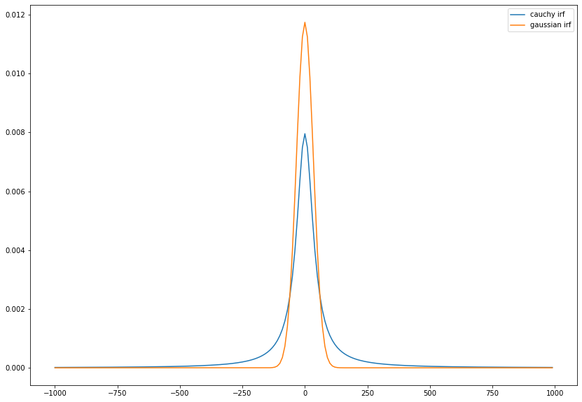
Compare cauchy and gaussian IRF with same fwhm
fwhm = 0.15 # 150 fs
t = np.linspace(-1,1,200)
cauchy = cauchy_irf(t,fwhm)
gau = gau_irf(t,fwhm)
plt.plot(t, cauchy, label='cauchy irf')
plt.plot(t, gau, label='gaussian irf')
plt.legend()
plt.show()
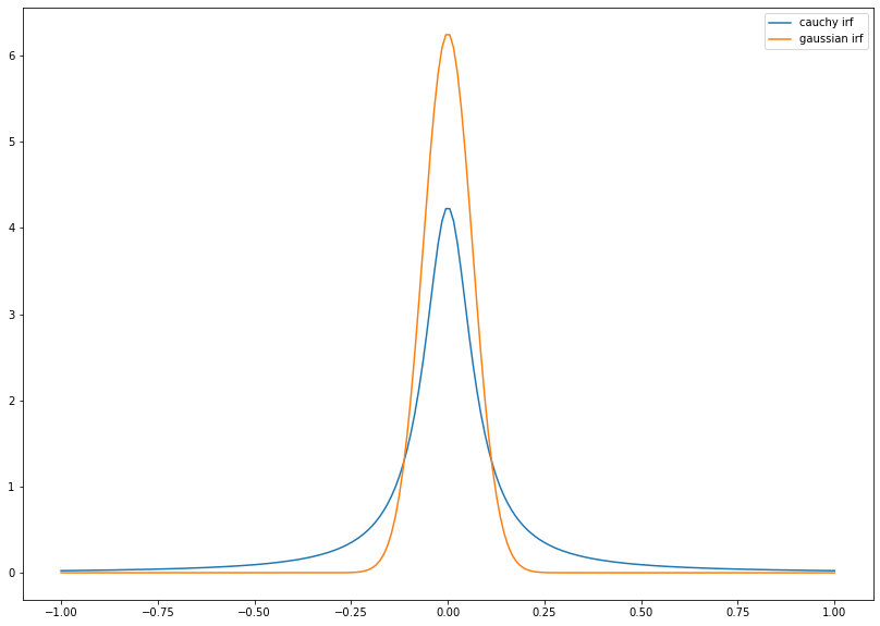
Cauchy irf is more diffuse then Gaussian irf
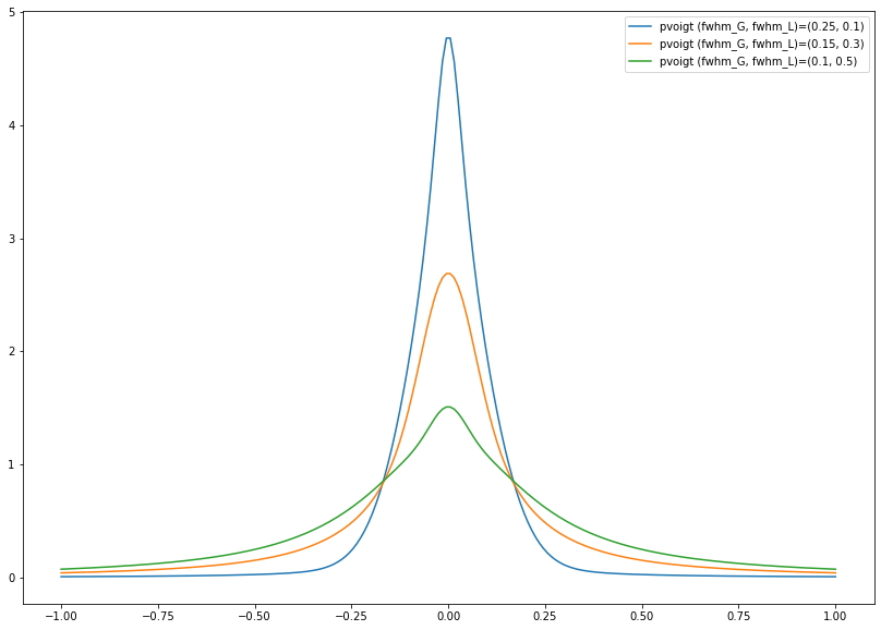
Compare pseudo voigt irf with different combination of (fwhm_G, fwhm_L)
(0.25, 0.1)
(0.15, 0.3)
(0.1, 0.5)
fwhm_1 = [0.25, 0.1]
fwhm_2 = [0.15, 0.3]
fwhm_3 = [0.1, 0.5]
eta_1 = calc_eta(fwhm_1)
eta_2 = calc_eta(fwhm_2)
eta_3 = calc_eta(fwhm_3)
pvoigt1 = pvoigt_irf(t, fwhm_1[0], fwhm_1[1], eta_1)
pvoigt2 = pvoigt_irf(t, fwhm_2[0], fwhm_2[1], eta_2)
pvoigt3 = pvoigt_irf(t, fwhm_3[0], fwhm_3[1], eta_3)
plt.plot(t, pvoigt1, label=f'pvoigt (fwhm_G, fwhm_L)=({fwhm_1[0]}, {fwhm_1[1]})')
plt.plot(t, pvoigt2, label=f'pvoigt (fwhm_G, fwhm_L)=({fwhm_2[0]}, {fwhm_2[1]})')
plt.plot(t, pvoigt3, label=f'pvoigt (fwhm_G, fwhm_L)=({fwhm_3[0]}, {fwhm_3[1]})')
plt.legend()
plt.show()
Compare baseline signal (IRF: cauchy, gaussian with same fwhm=0.15)
fwhm = np.array([0.15])
tau = np.zeros(0)
c = np.ones(1)
cauchy_baseline = model_n_comp_conv(t, fwhm, tau, c, base=True, irf='c')
gauss_baseline = model_n_comp_conv(t, fwhm, tau, c, base=True, irf='g')
plt.plot(t, cauchy_baseline, label='cauchy baseline')
plt.plot(t, gauss_baseline, label='gaussian baseline')
plt.legend()
plt.show()
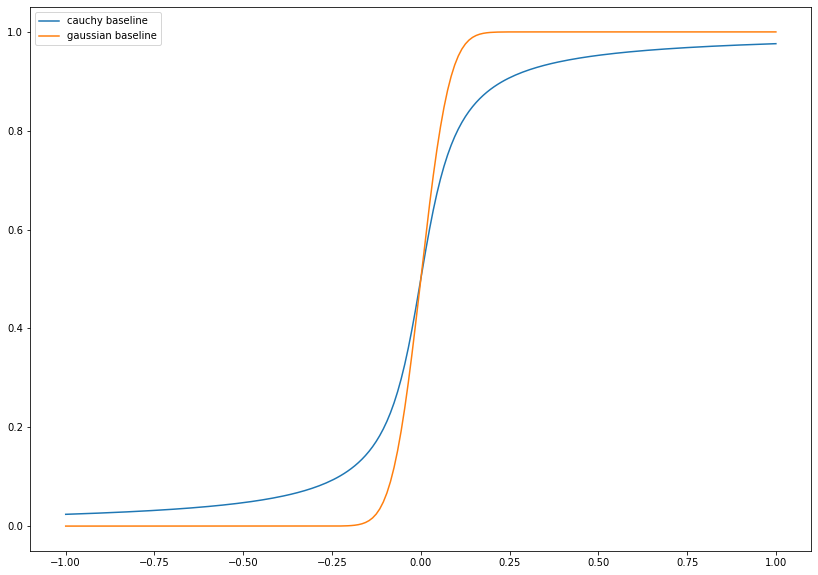
gaussian baseline is sharper than cauchy baseline
Compare pseudo voigt irf baseline signal with different combination of (fwhm_G, fwhm_L)
(0.25, 0.1)
(0.15, 0.3)
(0.1, 0.5)
fwhm_1 = [0.25, 0.1]
fwhm_2 = [0.15, 0.3]
fwhm_3 = [0.1, 0.5]
tau = np.zeros(0)
c = np.ones(1)
pv1_baseline = model_n_comp_conv(t, fwhm_1, tau, c, base=True, irf='pv')
pv2_baseline = model_n_comp_conv(t, fwhm_2, tau, c, base=True, irf='pv')
pv3_baseline = model_n_comp_conv(t, fwhm_3, tau, c, base=True, irf='pv')
plt.plot(t, pv1_baseline, label=f'pvoigt baseline (fwhm_G, fwhm_L)=({fwhm_1[0]}, {fwhm_1[1]})')
plt.plot(t, pv2_baseline, label=f'pvoigt baseline (fwhm_G, fwhm_L)=({fwhm_2[0]}, {fwhm_2[1]})')
plt.plot(t, pv3_baseline, label=f'pvoigt baseline (fwhm_G, fwhm_L)=({fwhm_3[0]}, {fwhm_3[1]})')
plt.legend()
plt.show()
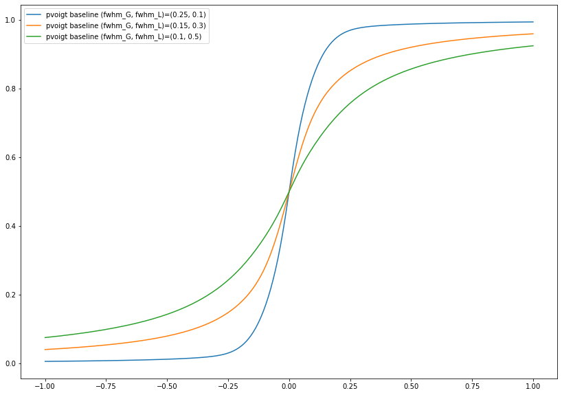
As lorenzian (cauchy) character smaller, sharper the baseline.
Compare exponential decay convolved with irf(cauchy, gaussian) with (tau=fwhm/2)
fwhm = np.array([0.15])
tau = np.array([fwhm[0]/2])
c = np.ones(1)
cauchy_expdecay = model_n_comp_conv(t, fwhm, tau, c, base=False, irf='c')
gauss_expdecay = model_n_comp_conv(t, fwhm, tau, c, base=False, irf='g')
plt.plot(t, cauchy_expdecay, label='cauchy exponential decay with tau=fwhm/2')
plt.plot(t, gauss_expdecay, label='gaussian expoential decay with tau=fwhm/2')
plt.legend()
plt.show()
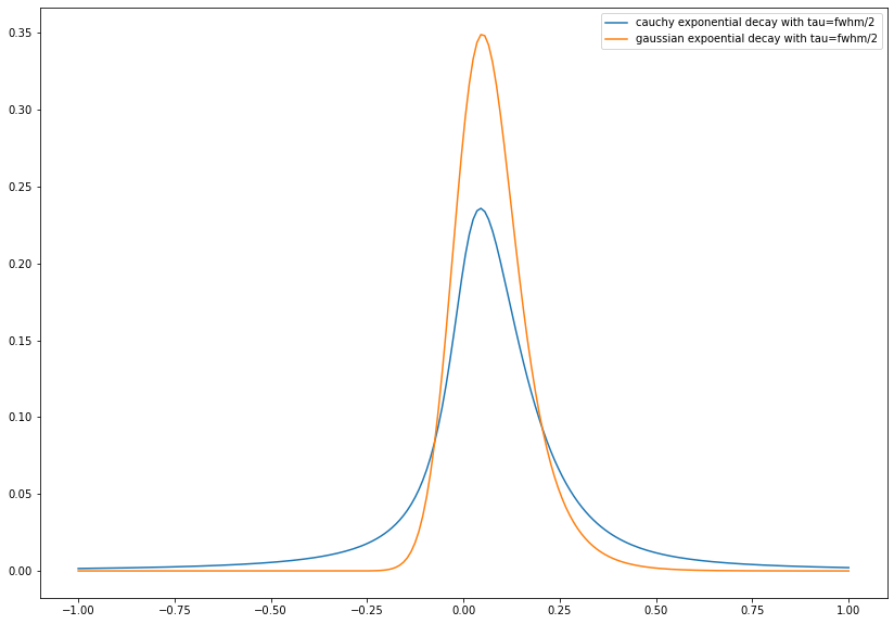
if tau: time constant is less than irf, we can only see little portion of exponetial decay feature.
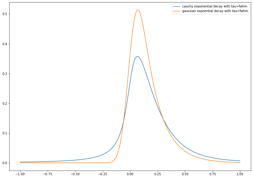
Compare exponential decay convolved with irf(cauchy, gaussian) with (tau=fwhm)
fwhm = np.array([0.15])
tau = np.array([fwhm[0]])
c = np.ones(1)
cauchy_expdecay = model_n_comp_conv(t, fwhm, tau, c, base=False, irf='c')
gauss_expdecay = model_n_comp_conv(t, fwhm, tau, c, base=False, irf='g')
plt.plot(t, cauchy_expdecay, label='cauchy exponential decay with tau=fwhm')
plt.plot(t, gauss_expdecay, label='gaussian expoential decay with tau=fwhm')
plt.legend()
plt.show()
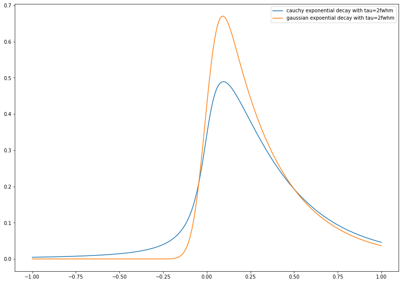
Compare exponential decay convolved with irf(cauchy, gaussian) with (tau=2fwhm)
fwhm = np.array([0.15])
tau = np.array([2*fwhm[0]])
c = np.ones(1)
cauchy_expdecay = model_n_comp_conv(t, fwhm, tau, c, base=False, irf='c')
gauss_expdecay = model_n_comp_conv(t, fwhm, tau, c, base=False, irf='g')
plt.plot(t, cauchy_expdecay, label='cauchy exponential decay with tau=2fwhm')
plt.plot(t, gauss_expdecay, label='gaussian expoential decay with tau=2fwhm')
plt.legend()
plt.show()
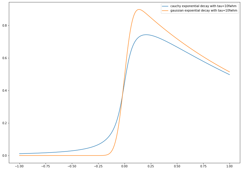
Compare exponential decay convolved with irf(cauchy, gaussian) with (tau=10fwhm)
fwhm = np.array([0.15])
tau = np.array([10*fwhm[0]])
c = np.ones(1)
cauchy_expdecay = model_n_comp_conv(t, fwhm, tau, c, base=False, irf='c')
gauss_expdecay = model_n_comp_conv(t, fwhm, tau, c, base=False, irf='g')
plt.plot(t, cauchy_expdecay, label='cauchy exponential decay with tau=10fwhm')
plt.plot(t, gauss_expdecay, label='gaussian expoential decay with tau=10fwhm')
plt.legend()
plt.show()
Compare exponential decay convolved with irf(cauchy, gaussian) with (tau=0.1fwhm)
fwhm = np.array([0.15])
tau = np.array([0.1*fwhm[0]])
c = np.ones(1)
cauchy_expdecay = model_n_comp_conv(t, fwhm, tau, c, base=False, irf='c')
gauss_expdecay = model_n_comp_conv(t, fwhm, tau, c, base=False, irf='g')
plt.plot(t, cauchy_expdecay, label='cauchy exponential decay with tau=fwhm/10')
plt.plot(t, gauss_expdecay, label='gaussian expoential decay with tau=fwhm/10')
plt.legend()
plt.show()
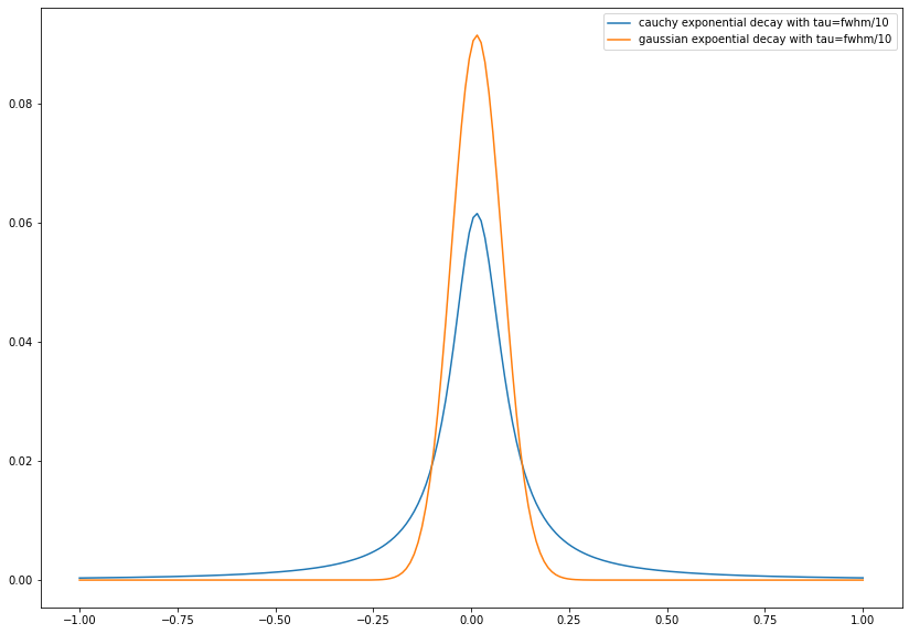
signal is very small and we can only see irf feature.
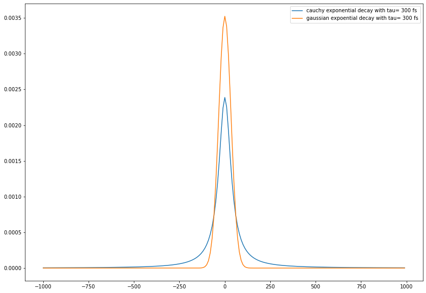
3rd generation x-ray source with fs dynamics
fwhm = 80 ps
tau1 = 300 fs
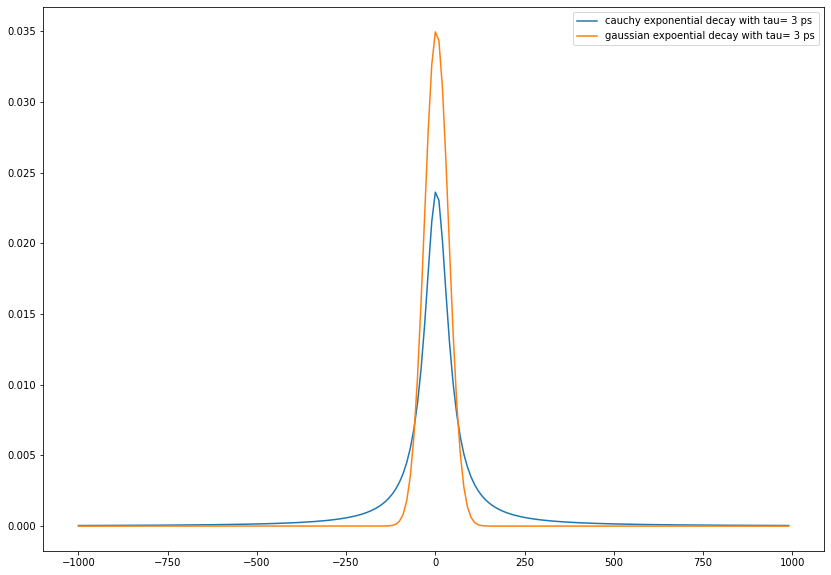
tau2 = 3 ps
tau3 = 30 ps
fwhm = 80 # 80 ps
t = np.arange(-1000, 1000, 10)
cauchy = cauchy_irf(t,fwhm)
gau = gau_irf(t,fwhm)
plt.plot(t, cauchy, label='cauchy irf')
plt.plot(t, gau, label='gaussian irf')
plt.legend()
plt.show()
fwhm = np.array([fwhm])
tau = np.array([0.3])
c = np.ones(1)
cauchy_expdecay = model_n_comp_conv(t, fwhm, tau, c, base=False, irf='c')
gauss_expdecay = model_n_comp_conv(t, fwhm, tau, c, base=False, irf='g')
plt.plot(t, cauchy_expdecay, label='cauchy exponential decay with tau= 300 fs')
plt.plot(t, gauss_expdecay, label='gaussian expoential decay with tau= 300 fs')
plt.legend()
plt.show()
tau = np.array([3])
c = np.ones(1)
cauchy_expdecay = model_n_comp_conv(t, fwhm, tau, c, base=False, irf='c')
gauss_expdecay = model_n_comp_conv(t, fwhm, tau, c, base=False, irf='g')
plt.plot(t, cauchy_expdecay, label='cauchy exponential decay with tau= 3 ps')
plt.plot(t, gauss_expdecay, label='gaussian expoential decay with tau= 3 ps')
plt.legend()
plt.show()
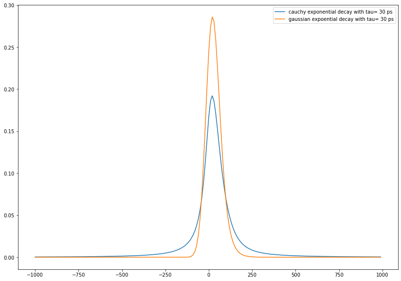
tau = np.array([30])
c = np.ones(1)
cauchy_expdecay = model_n_comp_conv(t, fwhm, tau, c, base=False, irf='c')
gauss_expdecay = model_n_comp_conv(t, fwhm, tau, c, base=False, irf='g')
plt.plot(t, cauchy_expdecay, label='cauchy exponential decay with tau= 30 ps')
plt.plot(t, gauss_expdecay, label='gaussian expoential decay with tau= 30 ps')
plt.legend()
plt.show()
Conclusion
3rd gen X-ray source with 80 ps fwhm could not see fs dynamics.