fit_seq Basic Example

Basic usage example for fit_seq utility. Yon can find example file from TRXASprefitpack-example fit_seq subdirectory.

1. In fit_seq sub directory you can find example_1.txt, example_2.txt, example_3.txt, example_4.txt files. These examples are generated from rate equation example section 1. sequential decay with varying time zero of each scan around -150 ps.

2. Type fit_seq -h Then it prints help message. You can find detailed description of arguments in the utility section of this document.

3. Type fit_seq example -sdt 1 --irf g --fwhm_G 100 -t0 -150 -150 -150 -150 --tau 500 10000 --no_base The first and the only one positional argument is prefix of time delay scan file to read. In this example you set four initial time zero parameter -t0 -150 -150 -150 -150, so it searchs example_1.txt,…,example_4.txt files and read them all. If you set one initial time zero parameter like -t0 -150 then it reads only one file example_1.txt even though there are four of files whoose prefix is example. First optional argument -sdt or --seq_decay_type sets the type of sequential decay. In this example we set --sdt 1, no raising. Second optional argument --irf set temporal shape of probe pulse. In this example we set --irf to g, gaussian shape. Third optional argument --fwhm_G is initial full width and half maximum of temporal shape of probe pulse. Since we use gaussian shape irf, we need to set initial fwhm_G. Fourth optional argument is --tau initial lifetime constant for each decay. In this example we set two decay lifetime component with initial value 500, 10000 respectively. If --no_base is not set, it will use infinite life time component to fit long lived spectral feature (eventhough it does not exist). Thus if you think there is not long lived spectral feature in your time delay scan result please set --no_base option to avoid over fitting.

4. After fitting process is finished, you can see both fitting result plot and report for fitting result in the console. Upper part of plot shows fitting curve and experimental data. Lower part of plot shows residual of fit (data-fit).

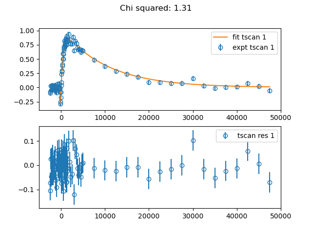
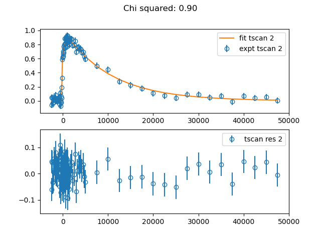
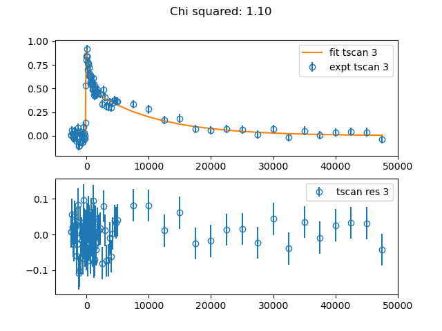
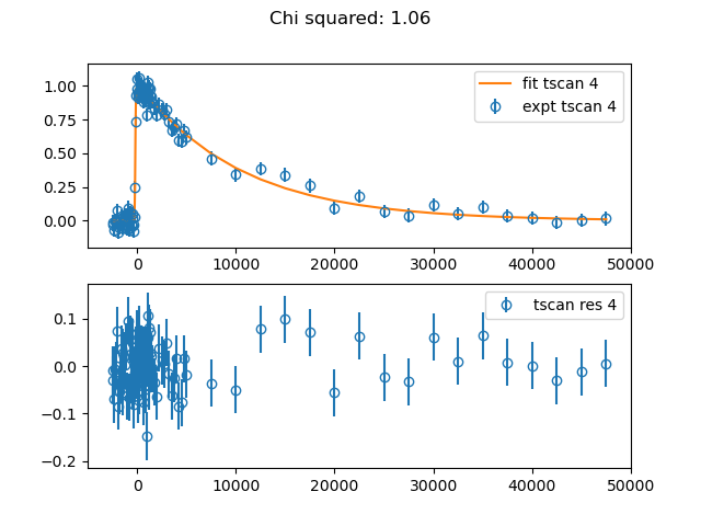
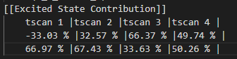
• In the excited state contribution section in the fitting result report, you can find contribution of each excited state in each time delay scan.

• Close all fitting result plot windows then example_abs.txt, example_fit.txt, example_fit_report.txt and example_res_i.txt files will be generated.

example_abs.txt contains coefficient of each excited states in each time delay scan

example_fit.txt contains fitting curve of time delay scan

example_fit_report.txt contains fitting result report.

example_res_i.txt contains residual of time delay scan (data-fit)