Rate Equation#

Objective#

Define equation
Solve equation
Compute model and signal

Note

In this example, we only deal with gaussian and cauchy irf with same fwhm

# import needed module
import numpy as np
import matplotlib.pyplot as plt
from TRXASprefitpack import solve_model, compute_model, compute_signal_gau
from TRXASprefitpack import compute_signal_cauchy, compute_signal_pvoigt
plt.rcParams["figure.figsize"] = (14,10)

basic information of functions#

help(solve_model)

Help on function solve_model in module TRXASprefitpack.mathfun.rate_eq:

solve_model(equation, y0)
    Solve system of first order rate equation
    
    
    :param equation: matrix corresponding to model
    :type equation: numpy_nd_array
    :param y0: initial condition
    :type y0: numpy_1d_array
    
    
    :return: eigenvalue of equation
    :rtype: numpy_1d_array
    :return: eigenvectors for equation
    :rtype: numpy_nd_array
    :return: coefficient where y_0 = Vc
    :rtype: numpy_1d_array

help(compute_model)

Help on function compute_model in module TRXASprefitpack.mathfun.rate_eq:

compute_model(t, eigval, V, c)
    Compute solution of the system of rate equations solved by solve_model
    Note: eigval, V, c should be obtained from solve_model
    
    
    :param t: time
    :type t: numpy_1d_array
    :param eigval: eigenvalue for equation
    :type eigval: numpy_1d_array
    :param V: eigenvectors for equation
    :type V: numpy_nd_array
    :param c: coefficient
    :type c: numpy_1d_array
    
    
    :return: solution of rate equation
    :rtype: numpy_nd_array

help(compute_signal_gau)

Help on function compute_signal_gau in module TRXASprefitpack.mathfun.rate_eq:

compute_signal_gau(t, fwhm, eigval, V, c)
    Compute solution of the system of rate equations solved by solve_model
    convolved with normalized gaussian distribution
    Note: eigval, V, c should be obtained from solve_model
    
    
    :param t: time
    :type t: numpy_1d_array
    :param fwhm: full width at half maximum of x-ray temporal pulse
    :type fwhm: float
    :param eigval: eigenvalue for equation
    :type eigval: numpy_1d_array
    :param V: eigenvectors for equation
    :type V: numpy_nd_array
    :param c: coefficient
    :type c: numpy_1d_array
    
    
    :return: 
     solution of rate equation convolved with normalized gaussian distribution
    :rtype: numpy_nd_array

help(compute_signal_cauchy)

Help on function compute_signal_cauchy in module TRXASprefitpack.mathfun.rate_eq:

compute_signal_cauchy(t, fwhm, eigval, V, c)
    Compute solution of the system of rate equations solved by solve_model
    convolved with normalized cauchy distribution
    Note: eigval, V, c should be obtained from solve_model
    
    
    :param t: time
    :type t: numpy_1d_array
    :param fwhm: full width at half maximum of x-ray temporal pulse
    :type fwhm: float
    :param eigval: eigenvalue for equation
    :type eigval: numpy_1d_array
    :param V: eigenvectors for equation
    :type V: numpy_nd_array
    :param c: coefficient
    :type c: numpy_1d_array
    
    
    :return: 
     solution of rate equation convolved with normalized cachy distribution
    :rtype: numpy_nd_array

help(compute_signal_pvoigt)

Help on function compute_signal_pvoigt in module TRXASprefitpack.mathfun.rate_eq:

compute_signal_pvoigt(t, fwhm_G, fwhm_L, eta, eigval, V, c)
    Compute solution of the system of rate equations solved by solve_model
    convolved with normalized pseudo voigt profile
    (:math:`pvoigt = (1-\eta) G(t) + \eta L(t)`,
    G(t): stands for normalized gaussian
    L(t): stands for normalized cauchy(lorenzian) distribution)
    
    Note: eigval, V, c should be obtained from solve_model
    
    :param t: time
    :type t: numpy_1d_array
    :param fwhm_G: 
     full width at half maximum of x-ray temporal pulse (gaussian part)
    :type fwhm_G: float
    :param fwhm_L:
     full width at half maximum of x-ray temporal pulse (lorenzian part)
    :type fwhm_L: float
    :param float eta: mixing parameter :math:`(0 < \eta < 1)`
    
    :type eta: float
    :param eigval: eigenvalue for equation
    :type eigval: numpy_1d_array
    :param V: eigenvectors for equation
    :type V: numpy_nd_array
    :param c: coefficient
    :type c: numpy_1d_array
    
    :return: 
     solution of rate equation convolved with normalized pseudo voigt profile
    :rtype: numpy_nd_array

Define equation#

Note

In pump-probe time resolved spectroscopy, the concentration of ground state is not much important. Only, the concentration of excited species are matter.

Consider model

'''
    k1     k2
A  ---> B ---> GS
y1: A
y2: B
y3: GS
'''

with initial condition

\[\begin{equation*} y(t) = \begin{cases} (0, 0, 1) & \text{if $t < 0$}, \\ (1, 0, 0) & \text{if $t=0$}. \end{cases} \end{equation*}\]

Then what we need to solve is

\[\begin{equation*} y'(t) = \begin{cases} (0, 0, 0) & \text{if $t < 0$}, \\ Ay(t) & \text{if $t \geq 0$} \end{cases} \end{equation*}\]

with $y(0)=y_0$.

Where $A$ is

\[\begin{equation*} A = \begin{pmatrix} -k_1 & 0 & 0 \\ k_1 & -k_2 & 0 \\ 0 & k_2 & 0 \end{pmatrix} \end{equation*}\]

# set lifetime tau1 = 10 ps, tau2 = 1 ns
# set fwhm of IRF = 1 ps

tau1 = 10
tau2 = 1000
fwhm = 1

# initial condition
y0 = np.array([1, 0, 0])

# set time range
t_short = np.arange(-10,50,0.1)
t_long = np.arange(-200,5000,10)

# Define equation
equation = np.array([[-1/tau1, 0, 0],
                    [1/tau1, -1/tau2, 0],
                    [0, 1/tau2, 0]])

# Solve equation
eigval, V, c = solve_model(equation, y0)

# Now compute model
y_short = compute_model(t_short, eigval, V, c)
y_long = compute_model(t_long, eigval, V, c)

#Next compute signal (model convolved with irf)
signal_short = compute_signal_gau(t_short, fwhm, eigval, V, c)
signal_long = compute_signal_gau(t_long, fwhm, eigval, V, c)
signal_short_cauchy = compute_signal_cauchy(t_short, fwhm, eigval, V, c)
signal_long_cauchy = compute_signal_cauchy(t_long, fwhm, eigval, V, c)

# since, y_1 + y_2 + y_3 = 1 for all t,
# y3 = 1 - (y_1+y_2)

y_short[-1, :] = 1 - (y_short[0, :] + y_short[1, :])
y_long[-1, :] = 1 - (y_long[0, :] + y_long[1, :])
signal_short[-1, :] = 1 - (signal_short[0, :] + signal_short[1, :])
signal_long[-1, :] = 1 - (signal_long[0, :] + signal_long[1, :])
signal_short_cauchy[-1, :] = 1 - (signal_short_cauchy[0, :] + signal_short_cauchy[1, :])
signal_long_cauchy[-1, :] = 1 - (signal_long_cauchy[0, :] + signal_long_cauchy[1, :])

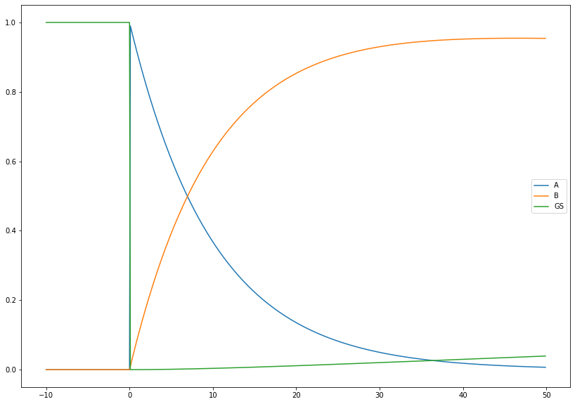
plot model#

short range

plt.plot(t_short, y_short[0, :], label='A')
plt.plot(t_short, y_short[1, :], label='B')
plt.plot(t_short, y_short[2, :], label='GS')
plt.legend()
plt.show()

png

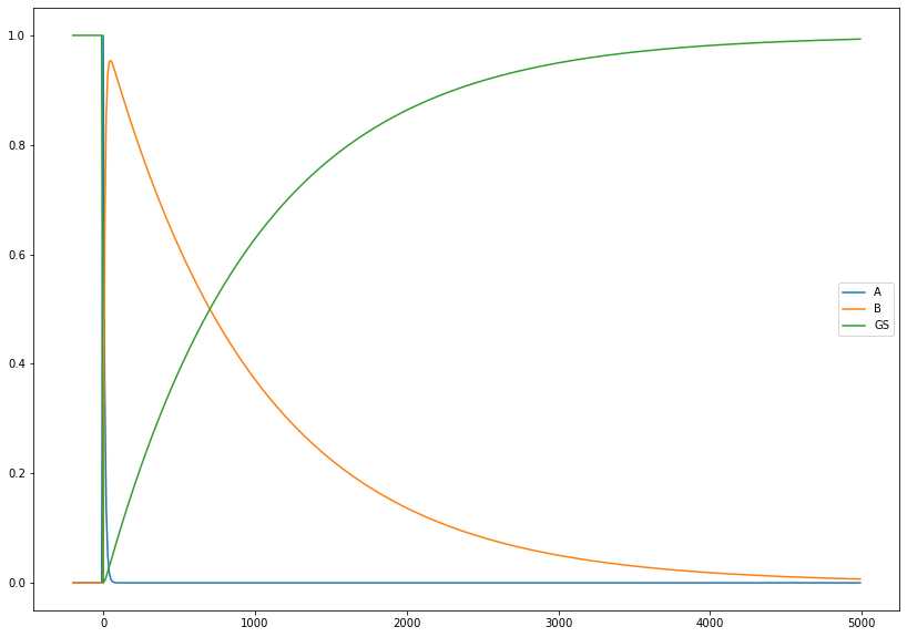
long range

plt.plot(t_long, y_long[0, :], label='A')
plt.plot(t_long, y_long[1, :], label='B')
plt.plot(t_long, y_long[2, :], label='GS')
plt.legend()
plt.show()

png

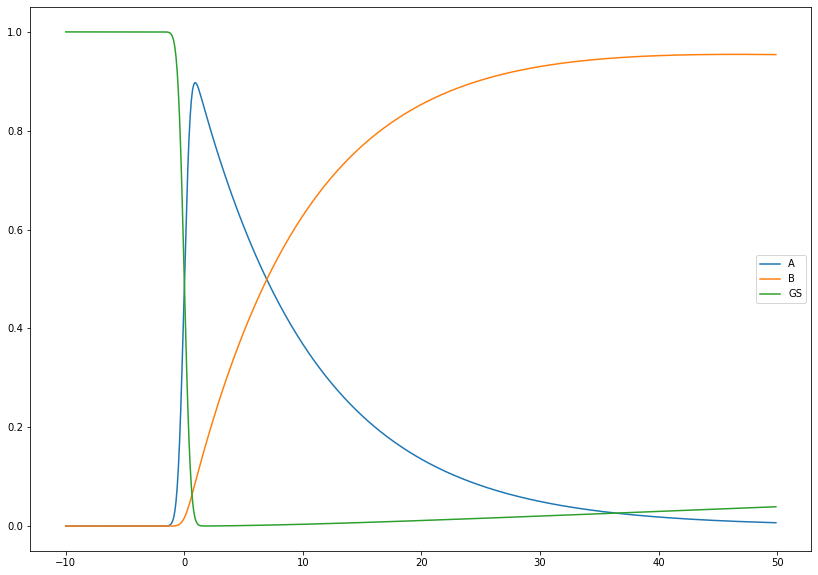
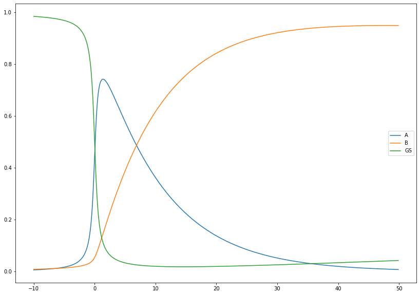
plot signal (gaussian)#

short range

plt.plot(t_short, signal_short[0, :], label='A')
plt.plot(t_short, signal_short[1, :], label='B')
plt.plot(t_short, signal_short[2, :], label='GS')
plt.legend()
plt.show()

png

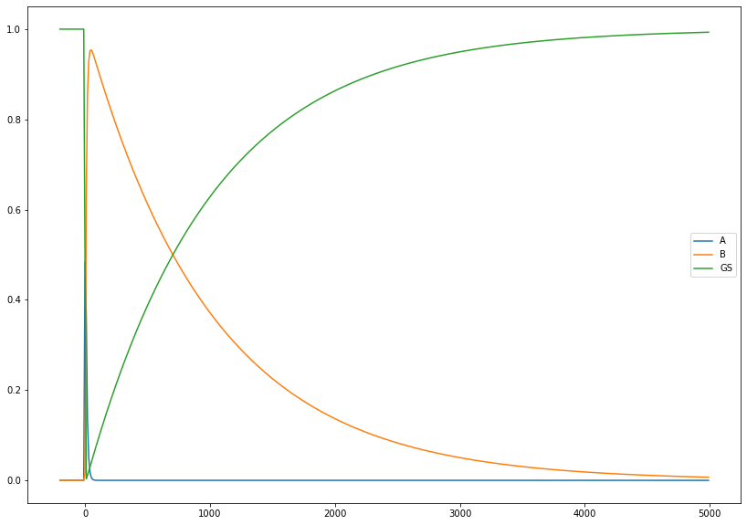
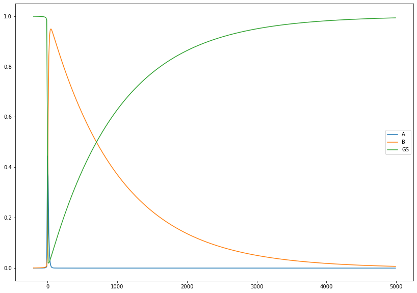
long range

plt.plot(t_long, signal_long[0, :], label='A')
plt.plot(t_long, signal_long[1, :], label='B')
plt.plot(t_long, signal_long[2, :], label='GS')
plt.legend()
plt.show()

png

plot signal (Cauchy)#

short range

plt.plot(t_short, signal_short_cauchy[0, :], label='A')
plt.plot(t_short, signal_short_cauchy[1, :], label='B')
plt.plot(t_short, signal_short_cauchy[2, :], label='GS')
plt.legend()
plt.show()

png

long range

plt.plot(t_long, signal_long_cauchy[0, :], label='A')
plt.plot(t_long, signal_long_cauchy[1, :], label='B')
plt.plot(t_long, signal_long_cauchy[2, :], label='GS')
plt.legend()
plt.show()

png

Conclusion#

IRF broads the signal
At short range, gaussian signal is much sharper than cauchy signal.
At long range, gaussian signal and cauchy signal look similar.

TRXASprefitpack 0.4.10 documentation

Rate Equation

Contents

Rate Equation#

Objective#

basic information of functions#

Define equation#

plot model#

plot signal (gaussian)#

plot signal (Cauchy)#

Conclusion#