fit_tscan Basic Example
Basic usage example for fit_tscan utility. Yon can find example file from TRXASprefitpack-example fit_tscan subdirectory.
Go to
basicsub directory offit_tscandirectory.In
basicsub directory, you can findexample_basic_1.txt,example_basic_2.txt,example_basic_3.txt,example_basic_4.txtfiles. These examples are generated from Library example, fitting with time delay scan (model: exponential decay).Type
fit_tscan -hThen it prints help message. You can find detailed description of arguments in the utility section of this document.First try single decay model.
Type
fit_tscan example_basic --num_file 4 --mode decay --irf g --fwhm_G 150 -t0 0 0 0 0 --tau 15000 --no_base -o decay_1The first and the only one positional argument is prefix of time delay scan file to read. In this example you set--num_file 4and four initial time zero parameter0 0 0 0, so it searchsexample_basic_1.txt,…,example_basic_4.txtfiles and read them all.
Second optional argument --mode sets fitting model, we set --mode decay that is fitting with convolution of exponential decay and instrumental response function.
Third optional argument --irf sets temporal shape of probe pulse. In this example we set --irf to g, gaussian shape.
Fourth optional argument --fwhm_G is initial full width and half maximum of temporal shape of probe pulse. Since we use gaussian shape irf, we need to set initial fwhm_G.
Fifth optional argument is -t0 initial guess for time zero of each time delay scan.
Sixth optional argument is --tau initial guess for lifetime of decay component. In this example we use one decay exponential function with initial value 15000.
If --no_base is not set, it will use infinite life time component to fit long lived spectral feature (eventhough it does not exist). Thus if you think there is no long lived spectral feature in your time delay scan result please set --no_base option to avoid over fitting.
Last optional argument is -o it sets name of hdf5 file to save fitting result and directory to save text file format of fitting result.
After fitting process is finished, you can see both fitting result plot and report for fitting result in the console. Upper part of plot shows fitting curve and experimental data. Lower part of plot shows residual of fit (data-fit).
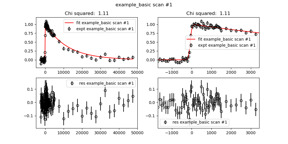

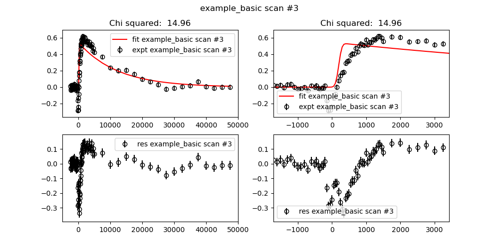
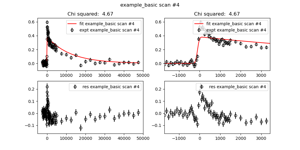
Optionally you can set
--save_figto save figure to directory set by-ooption, instead of display.Based on residual plot, there exists short lived decay component, now try with your self to add one or two more decay component.
For robust fitting result you can turn on global optimization algorithm
ampgoorbasinhoppingby setting--method_glboption.You can further analysis fitting result with
decay_1.h5file.
Description for Output file in decay_1 directory.
weight_example_basic.txtcontains coefficient of each component in each time delay scanfit_example_basic.txtcontains fitting curve of time delay scanfit_summary.txtSummary of fitting result.res_example_basic_i.txtcontains residual of time delay scan (data-fit)